6.3: The Kolmogorov Differential Equations

Let \(P_{ij} (t)\) be the probability that a Markov process {\(X(t); t \geq 0\)} is in state \(j\) at time \(t\) given that \(X(0) = i\),

\[ P_{ij}(t) = P\{X(t)=j|X(0)=i \} \nonumber \]

\(P_{ij} (t)\) is analogous to the \(n^{th}\) order transition probabilities \(P_{ij}^n\) for Markov chains. We have already seen that \(\lim_{t\rightarrow \infty} P_{ij} \ref{t} = p_j\) for the case where the embedded chain is positive recurrent and \(\sum_i \pi_i/\nu_i < \infty\). Here we want to find the transient behavior, and we start by deriving the Chapman-Kolmogorov equations for Markov processes. Let \(s\) and \(t\) be arbitrary times, \(0 < s < t\). By including the state at time \(s\), we can rewrite (6.3.1) as

\[ \begin{align} P_{ij}(t) \quad &= \quad \sum_k \text{Pr}\{X(t)=j, \, X(s)=k|X(0)=i \} \nonumber \\ &= \quad \sum_k \text{Pr} \{X(s)=k | X(0)=i\} \, \, \text{Pr}\{X(t)=j |X(s)=k \} ; \qquad \text{all }i,j \end{align} \nonumber \]

where we have used the Markov condition, (6.1.3). Given that \(X(s) = k\), the residual time until the next transition after \(s\) is exponential with rate \(\nu_k\), and thus the process starting at time \(s\) in state \(k\) is statistically identical to that starting at time 0 in state \(k\). Thus, for any \(s\), \(0 \leq s \leq t\), we have

\[ P\{ X(t)=j | X(s)=k \} = P_{kj} (t-s) \nonumber \]

Substituting this into (6.3.2), we have the Chapman-Kolmogorov equations for a Markov process,

\[ P_{ij}(t) = \sum_k P_{ik}(s)P_{kj}(t-s) \nonumber \]

These equations correspond to \ref{3.8} for Markov chains. We now use these equations to derive two types of sets of di↵erential equations for \(P_{ij} (t)\). The first are called the Kolmogorov forward differential equations, and the second the Kolmogorov backward differential equations. The forward equations are obtained by letting \(s\) approach \(t\) from below, and the backward equations are obtained by letting \(s\) approach 0 from above. First we derive the forward equations.

For \(t- s\) small and positive, \(P_{kj} (t- s)\) in (6.3.3) can be expressed as \((t-s)q_{kj} + o(t-s)\) for \(k \neq j\). Similarly, \(P_{jj} (t- s)\) can be expressed as \(1 -(t-s)\nu_j + o(s)\). Thus (6.3.3) becomes

\[ P_{ij}(t)=\sum_{k\neq j} [P_{ik}(s)(t-s) q_{kj}] + P_{ij}(s)[1-(t-s)\nu_j] + o(t-s) \nonumber \]

We want to express this, in the limit \(s \rightarrow t\), as a differential equation. To do this, subtract \(P_{ij} (s)\) from both sides and divide by \(t- s\).

\[ \dfrac{P_{ij}(t)-P_{ij}(s)}{t-s} = \sum_{k\neq j} (P_{ik}(s)q_{kj})-P_{ij}(s)\nu_j+\dfrac{o(s)}{s} \nonumber \]

Taking the limit as \(s \rightarrow t\) from below,¹ we get the Kolmogorov forward equations,

\[ \dfrac{dP_{ij}(t)}{dt} = \sum_{k\neq j} (P_{ik}(t)q_{kj})-P_{ij}(t)\nu_j \nonumber \]

The first term on the right side of (6.3.5) is the rate at which transitions occur into state \(j\) at time \(t\) and the second term is the rate at which transitions occur out of state \(j\). Thus the difference of these terms is the net rate at which transitions occur into \(j\), which is the rate at which \(P_{ij} (t)\) is increasing at time \(t\).

Example 6.3.1 (A queueless M/M/1 queue) Consider the following 2-state Markov process where \(q_{01} = \lambda\) and \(q_{10} = µ\).

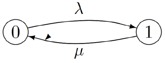
This can be viewed as a model for an M/M/1 queue with no storage for waiting customers. When the system is empty (state 0), memoryless customers arrive at rate \(\lambda\), and when the server is busy, an exponential server operates at rate \(µ\), with the system returning to state 0 when service is completed.

To find \(P_{01}(t)\), the probability of state 1 at time \(t\) conditional on state 0 at time 0, we use the Kolmogorov forward equations for \(P_{01}(t)\), getting

\[ \dfrac{dP_{01}(t)}{dt} = P_{00}(t) q_{01}-P_{01}(t)\nu_1 = P_{00}(t)\lambda -P_{01}(t)\mu \nonumber \]

Using the fact that \(P_{00}(t) = 1 -P_{01}(t)\), this becomes

\[ \dfrac{dP_{01}(t)}{dt} = \lambda -P_{01}(t)(\lambda+\mu) \nonumber \]

Using the boundary condition \(P_{01}(0) = 0\), the solution is

\[ P_{01}(t) = \dfrac{\lambda}{\lambda+\mu}\left[ 1-e^{-(\lambda+\mu)t}\right] \nonumber \]

Thus \(P_{01}(t)\) is 0 at \(t = 0\) and increases as \(t \rightarrow \infty\) to its steady-state value in state 1, which is \(\lambda/( \lambda+ µ)\).

In general, for any given starting state \(i\) in a Markov process with \(\mathsf{M}\) states, (6.3.5) provides a set of \(\mathsf{M}\) simultaneous linear differential equations, one for each \(j\), \(1\leq j \leq \mathsf{M}\). As we saw in the example, one of these is redundant because \(\sum^{\mathsf{M}}_{j=1} P_{ij} \ref{t} = 1\). This leaves \(\mathsf{M}- 1\) simultaneous linear differential equations to be solved.

For more than 2 or 3 states, it is more convenient to express (6.3.5) in matrix form. Let \([P(t)]\) (for each \(t > 0\)) be an \(\mathsf{M}\) by \(\mathsf{M}\) matrix whose \(i\), \(j\) element is \(P_{ij} (t)\). Let \([Q]\) be an \(\mathsf{M}\) by \(\mathsf{M}\) matrix whose \(i\), \(j\) element is \(q_{ij}\) for each \(i \neq j\) and \(-\nu_j\) for \(i = j\). Then (6.3.5) becomes

\[ \dfrac{d[P(t)]}{dt} = [P(t)][Q] \nonumber \]

For Example 6.3.1, \(P_{ij} (t)\) can be calculated for each \(i\), \(j\) as in (6.3.6), resulting in

\[ [P(t)] = \left[ \begin{array}{cc} \dfrac{\mu}{\lambda+\mu}+\dfrac{\lambda}{\lambda+\mu} e^{-(\lambda+\mu)t} & \dfrac{\lambda}{\lambda+\mu}-\dfrac{\lambda}{\lambda+\mu}e^{-(\lambda+\mu)t} \\ \dfrac{\mu}{\lambda+\mu} +\dfrac{\lambda}{\lambda+\mu}e^{-(\lambda+\mu)t} & \dfrac{\lambda}{\lambda+\mu}-\dfrac{\lambda}{\lambda+\mu}e^{-(\lambda+\mu)t} \end{array} \right] \qquad [Q] = \left[ \begin{array}{cc} -\lambda & \lambda \\ \\ \mu & -\mu \end{array} \right] \nonumber \]

In order to provide some insight into the general solution of (6.3.7), we go back to the sampled time approximation of a Markov process. With an increment of size \(\delta\) between samples, the probability of a transition from \(i\) to \(j\), \(i \neq j\), is \(q_{ij}\delta + o(\delta)\), and the probability of remaining in state \(i\) is \(1-\nu_i\delta +o(\delta)\). Thus, in terms of the matrix \([Q]\) of transition rates, the transition probability matrix in the sampled time model is \([I] + \delta[Q]\), where \([I]\) is the identity matrix. We denote this matrix by \([W_{\delta}] = [I]+\delta[Q]\). Note that \(\lambda\) is an eigenvalue of \([Q]\) if and only if \(1+\lambda\delta\) is an eigenvalue of \([W_{\delta}]\). Also the eigenvectors of these corresponding eigenvalues are the same. That is, if \(\boldsymbol{\nu}\) is a right eigenvector of \([Q]\) with eigenvalue \(\lambda\), then \(\boldsymbol{\nu}\) is a right eigenvector of \([W_{\delta}]\) with eigenvalue \(1 +\lambda \delta \), and conversely. Similarly, if \(\boldsymbol{p}\) is a left eigenvector of \([Q]\) with eigenvalue \(\lambda\), then \(\boldsymbol{p}\) is a left eigenvector of \([W_{\delta}]\) with eigenvalue \(1 +\lambda\delta \), and conversely.

We saw in Section 6.2.5 that the steady-state probability vector \(\boldsymbol{p}\) of a Markov process is the same as that of any sampled-time approximation. We have now seen that, in addition, all the eigenvectors are the same and the eigenvalues are simply related. Thus study of these di↵erential equations can be largely replaced by studying the sampled-time approximation.

The following theorem uses our knowledge of the eigenvalues and eigenvectors of transition matrices such as \([W_{\delta}]\) in Section 3.4, to be more specific about the properties of \([Q]\).

Theorem 6.3.1 Consider an irreducible finite-state Markov process with \(\mathsf{M}\) states. Then the matrix \([Q]\) for that process has an eigenvalue \(\lambda\) equal to 0. That eigenvalue has a right eigenvector \(e = (1, 1, . . . , 1)^{\mathsf{T}}\) which is unique within a scale factor. It has a left eigenvector \(\boldsymbol{p} = (p_1, . . . , p_{\mathsf{M}})\) that is positive, sums to 1, satisfies (6.2.17), and is unique within a scale factor. All the other eigenvalues of \([Q]\) have strictly negative real parts.

Proof: Since all \(\mathsf{M}\) states communicate, the sampled time chain is recurrent. From Theorem 3.4.1, \([W_{\delta}]\) has a unique eigenvalue \(\lambda= 1\). The corresponding right eigenvector is \(e\) and the left eigenvector is the steady-state probability vector \(\boldsymbol{p}\) as given in (3.9). Since \([W_{\delta}]\) is recurrent, the components of \(\boldsymbol{p}\) are strictly positive. From the equivalence of (6.2.17) and (6.2.18), \(\boldsymbol{p}\), as given by (6.2.17), is the steady-state probability vector of the process. Each eigenvalue \(\lambda_{\delta}\) of \([W_{\delta}]\) corresponds to an eigenvalue \(\lambda\) of \([Q]\) with the correspondence \(\lambda_{\delta}= 1+\lambda\delta\), \(i.e.\), \(\lambda= (\lambda_{\delta}-1)/\delta\). Thus the eigenvalue 1 of \([W_{\delta}]\) corresponds to the eigenvalue 0 of \([Q]\). Since \(|\lambda_{\delta}| \leq 1\) and \(\lambda_{\delta}\neq 1\) for all other eigenvalues, the other eigenvalues of \([Q]\) all have strictly negative real parts, completing the proof.

\(\square\)

We complete this section by deriving the Komogorov backward equations. For \(s\) small and positive, the Chapman-Kolmogorov equations in (6.3.3) become

\[ \begin{aligned} P_{ij}(t) \quad &= \quad \sum_kP_{ik}(s)P_{kj}(t-s) \\ &= \quad \sum_{k\neq i} sq_{ik}P_{kj} (t-s)+(1-s\nu_i)P_{ij}(t-s)+o(s) \end{aligned} \nonumber \]

Subtracting \(P_{ij} (t -s)\) from both sides and dividing by \(s\),

\[ \begin{align} \dfrac{P_{ij}(t)-P_{ij}(t-s)}{s} \quad &= \quad \sum_{k\neq i}q_{ik}P_{kj}(t-s)-\nu_iP_{ij}(t-s)+ \dfrac{o(s)}{s} \nonumber \\ \dfrac{dP_{ij}(t)}{dt} \quad &= \quad \sum_{k\neq i} q_{ik}P_{kj}(t)-\nu_iP_{ij}(t) \end{align} \nonumber \]

In matrix form, this is expressed as

\[ \dfrac{d[P(t)]}{dt} = [Q][P(t)] \nonumber \]

By comparing (6.3.9) and (6.3.7), we see that \([Q][P(t)] = [P(t)][Q]\), \(i.e.\), that the matrices \([Q]\) and \([P(t)]\) commute. Simultaneous linear differential equations appear in so many applications that we leave the further exploration of these forward and backward equations as simple differential equation topics rather than topics that have special properties for Markov processes.

_____________________________________________________________

1. We have assumed that the sum and the limit in (6.1.3) can be interchanged. This is certainly valid if the state space is finite, which is the only case we analyze in what follows.