6.5: Birth-Death Processes

Birth-death processes are very similar to the birth-death Markov chains that we studied earlier. Here transitions occur only between neighboring states, so it is convenient to define \(\lambda_i\) as \(q_{i,i+1}\) and \(μ_i\) as \(q_{i,i-1}\) (see Figure 6.9). Since the number of transitions from \(i\) to \(i + 1\) is within 1 of the number of transitions from \(i + 1\) to \(i\) for every sample path, we conclude that

\[p_i\lambda_i = p_{i+1}\mu_{i+1} \nonumber \]

This can also be obtained inductively from (6.2.17) using the same argument that we used earlier for birth-death Markov chains.

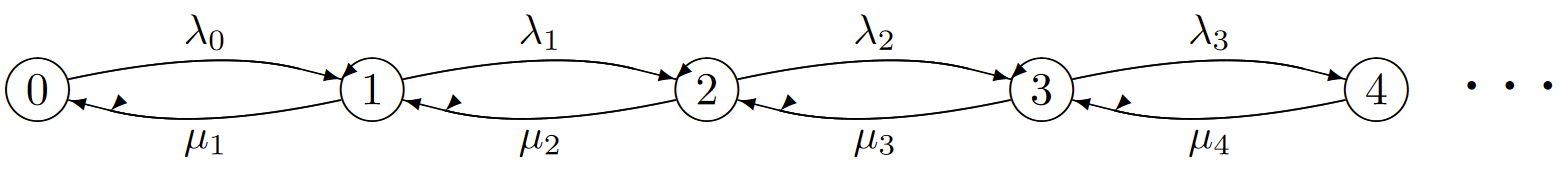
Figure 6.9: Birth-death process.

Define \(\rho_i\) as \(\lambda_i/\mu_{i+1}\). Then applying (6.5.1) iteratively, we obtain the steady-state equations

\[ p_i = p_0 \prod^{i-1}_{j=0} \rho_j ; \quad i\geq 1 \nonumber \]

We can solve for \(p_0\) by substituting (6.5.2) into \(\sum_i p_i\), yielding

\[ p_0 = \dfrac{1}{1+\sum^{\infty}_{i=1} \prod^{i-1}_{j=0} \rho_j } \nonumber \]

For the M/M/1 queue, the state of the Markov process is the number of customers in the system (\(i.e.\), customers either in queue or in service). The transitions from \(i\) to \(i + 1\) correspond to arrivals, and since the arrival process is Poisson of rate \(\lambda\), we have \(\lambda_i=\lambda\) for all \(i\geq 0\). The transitions from \(i\) to \(i-1\) correspond to departures, and since the service time distribution is exponential with parameter \(\mu\), say, we have \(\mu_i=\mu\) for all \(i\geq 1\). Thus, (6.5.3) simplifies to \(p_0=1-\rho\), where \(\rho=\lambda/\mu\) and thus

\[ p_i = (1-\rho) \rho^i; \qquad i\geq 0 \nonumber \]

We assume that \(\rho< 1\), which is required for positive recurrence. The probability that there are \(i\) or more customers in the system in steady state is then given by \(P \{X(t)\geq i\}=\rho^i\) and the expected number of customers in the system is given by

\[ \mathsf{E}[X(t)] = \sum^{\infty}_{i=1} P\{X(t)\geq i\} = \dfrac{\rho}{1-\rho} \nonumber \]

The expected time that a customer spends in the system in steady state can now be deter­mined by Little’s formula (Theorem 4.5.3).

\[ \mathsf{E}[\text{System time}]=\dfrac{\mathsf{E}[X(t)]}{\lambda} = \dfrac{\rho}{\lambda(1-\rho)}=\dfrac{1}{\mu-\lambda} \nonumber \]

The expected time that a customer spends in the queue (\(i.e.\), before entering service) is just the expected system time less the expected service time, so

\[ \mathsf{E}[\text{Queuing time}]=\dfrac{1}{\mu-\lambda}-\dfrac{1}{\mu} = \dfrac{\rho}{\mu-\lambda} \nonumber \]

Finally, the expected number of customers in the queue can be found by applying Little’s formula to (6.5.7),

\[ \mathsf{E} [\text{Number in queue}] = \dfrac{\lambda\rho}{\mu-\lambda} \nonumber \]

Note that the expected number of customers in the system and in the queue depend only on \(\rho\), so that if the arrival rate and service rate were both speeded up by the same factor, these expected values would remain the same. The expected system time and queuing time, however would decrease by the factor of the rate increases. Note also that as \(\rho\) approaches 1, all these quantities approach infinity as \(1/(1-\rho)\). At the value \(\rho = 1\), the embedded Markov chain becomes null-recurrent and the steady-state probabilities (both {\(\pi_i; i\geq 0\)} and {\(p_i; i\geq 0\)}) can be viewed as being all 0 or as failing to exist.

There are many types of queuing systems that can be modeled as birth-death processes. For example the arrival rate could vary with the number in the system and the service rate could vary with the number in the system. All of these systems can be analyzed in steady state in the same way, but (6.5.2) and (6.5.3) can become quite messy in these more complex systems. As an example, we analyze the M/M/m system. Here there are \(m\) servers, each with exponentially distributed service times with parameter \(μ\). When \(i\) customers are in the system, there are \(i\) servers working for \(i < m\) and all \(m\) servers are working for \(i\geq m\). With \(i\) servers working, the probability of a departure in an incremental time \(\delta\) is \(i\mu\delta\), so that \(μ_i\) is \(iμ\) for \(i < m\) and \(mμ\) for \(i\geq m\) (see Figure 6.10).

Define \(\rho = \lambda/(mμ)\). Then in terms of our general birth-death process notation, \(\rho_i = m\rho /(i + 1)\) for \(i < m\) and \(\rho_i = \rho\) for \(i\geq m\). From (6.5.2), we have

\[ \begin{align} p_i \quad &= \quad p_0 \dfrac{m\rho}{1}\dfrac{m\rho}{2} ... \dfrac{m\rho}{i} \quad = \quad \dfrac{p_0(m\rho)^i}{i!}; \qquad i\leq m \\ p_i \quad &= \quad \dfrac{p_0\rho^im^m}{m!} ; \qquad i\geq m \end{align} \nonumber \]

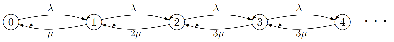
Figure 6.10: M/M/m queue for \( m = 3\).

We can find \(p_0\) by summing \(p_i\) and setting the result equal to 1; a solution exists if \(\rho< 1\). Nothing simplifies much in this sum, except that \(\sum_{i\geq m}p_i=p_0(\rho m)^m/[m!(1-\rho)]\), and the solution is

\[ p_0 = \left[ \dfrac{(m\rho)^m}{m!(1-\rho)} + \sum^{m-1}_{i=0} \dfrac{(m\rho)^i}{i!} \right]^{-1} \nonumber \]