6.6: Reversibility for Markov Processes

In Section 5.3 on reversibility for Markov chains, \ref{5.37} showed that the backward transition probabilities \(P_{ij}^*\) in steady state satisfy

\[ \pi_iP_{ij}^* = \pi_j P_{ji} \nonumber \]

These equations are then valid for the embedded chain of a Markov process. Next, consider backward transitions in the process itself. Given that the process is in state \(i\), the probability of a transition in an increment \(\delta\) of time is \(\nu_i\delta+o(\delta)\), and transitions in successive increments are independent. Thus, if we view the process running backward in time, the probability of a transition in each increment \(\delta\) of time is also \(\nu_i\delta+o(\delta)\) with independence between increments. Thus, going to the limit \(\delta\rightarrow 0\), the distribution of the time backward to a transition is exponential with parameter \(\nu_i\). This means that the process running backwards is again a Markov process with transition probabilities \(P_{ij}^*\) and transition rates \(\nu_i\). Figure 6.11 helps to illustrate this.

Since the steady-state probabilities {\(p_i; i\geq 0\)} for the Markov process are determined by

\[ p_i = \dfrac{\pi_i/\nu_i}{\sum_k \pi_k / \nu_k} \nonumber \]

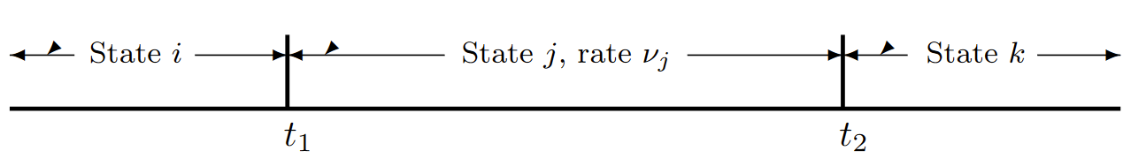
Figure 6.11: The forward process enters state \( j\) at time \(t_1\) and departs at \(t_2\). The backward process enters state \(j\) at time \(t_2\) and departs at \(t_1\). In any sample function, as illustrated, the interval in a given state is the same in the forward and backward process. Given \(X(t) = j\), the time forward to the next transition and the time backward to the previous transition are each exponential with rate \(\nu_j\).

and since \(\{\pi_i; i\geq 0\}\) and \(\{\nu_i;i\geq 0\}\) are the same for the forward and backward processes, we see that the steady-state probabilities in the backward Markov process are the same as the steady-state probabilities in the forward process. This result can also be seen by the correspondence between sample functions in the forward and backward processes.

The transition rates in the backward process are defined by \(q_{ij}^*= \nu_iP_{ij}^*\). Using (6.6.1), we have

\[ q_{ij}^* = \nu_jP_{ij}^* = \dfrac{\nu_i\pi_jP_{ij}}{\pi_i} = \dfrac{\nu_i\pi_jq_{ij}}{\pi_i \nu_j} \nonumber \]

From (6.6.2), we note that \(p_j = \alpha \pi_j /\nu_j\) and \(p_i = \alpha\pi_i/\nu_i\) for the same value of \(\alpha\). Thus the ratio of \(\pi_j /\nu_j\) to \(\pi_i/\nu_i\) is \(p_j /p_i\). This simplifies (6.6.3) to \(q_{ij}^*= p_j q_{ji}/p_i\), and

\[ p_iq_{ij}^*=p_jq_{ij} \nonumber \]

This equation can be used as an alternate definition of the backward transition rates. To interpret this, let \(\delta\) be a vanishingly small increment of time and assume the process is in steady state at time \(t\). Then \(\delta p_jq_{ij} \approx \text{Pr}\{X(t)=j\} \text{Pr} \{X(t+\delta)=i | X(t)=j\} \) whereas \(\delta p_iq_{ij}^* \approx \text{Pr}\{ X(t+\delta) = i\} \text{Pr}\{ X(t)=j | X(t+\delta ) =i \} \).

A Markov process is defined to be reversible if \(q_{ij}^*= q_{ij}\) for all \(i, j\). If the embedded Markov chain is reversible, (\(i.e.\), \(P_{ij}^*= P_{ij}\) for all \(i, j\)), then one can repeat the above steps using \(P_{ij}\) and \(q_{ij}\) in place of \(P_{ij}^*\) and \( q_{ij}^*\) to see that \(p_iq_{ij} = p_j q_{ji}\) for all \(i, j\). Thus, if the embedded chain is reversible, the process is also. Similarly, if the Markov process is reversible, the above argument can be reversed to see that the embedded chain is reversible. Thus, we have the following useful lemma.

Lemma 6.6.1. Assume that steady-state probabilities \(\{p_i; i\geq 0\}\) exist in an irreducible Markov process (\(i.e.\), (6.2.17) has a solution and \(\sum p_i\nu_i < \infty\)). Then the Markov process is reversible if and only if the embedded chain is reversible.

One can find the steady-state probabilities of a reversible Markov process and simultane­ously show that it is reversible by the following useful theorem (which is directly analogous to Theorem 5.3.2 of chapter 5).

Theorem 6.6.1. For an irreducible Markov process, assume that \(\{ p_i; i\geq 0\}\) is a set of nonnegative numbers summing to 1, satisfying \(\sum_i p_i\nu_i\leq \infty\), and satisfying

\[ p_iq_{ij} = p_jq_{ji} \qquad for \, all \, i,j \nonumber \]

Then \(\{ p_i;i\geq 0\}\) is the set of steady-state probabilities for the process, \(p_i > 0\) for all \(i\), the process is reversible, and the embedded chain is positive recurrent.

Proof: Summing (6.6.5) over \(i\), we obtain

\[ \sum_i p_iq_{ij} = p_j\nu_j \qquad \text{for all } j \nonumber \]

These, along with \(\sum_i p_i = 1\) are the steady-state equations for the process. These equations have a solution, and by Theorem 6.2.2, \(p_i > 0\) for all \(i\), the embedded chain is positive recurrent, and \(p_i = \lim_{t\rightarrow \infty} \text{Pr}\{X(t) = i\}\). Comparing (6.6.5) with (6.6.4), we see that \(q_{ij} = q_{ij}^*\), so the process is reversible.

\(\square \)

There are many irreducible Markov processes that are not reversible but for which the backward process has interesting properties that can be deduced, at least intuitively, from the forward process. Jackson networks (to be studied shortly) and many more complex networks of queues fall into this category. The following simple theorem allows us to use whatever combination of intuitive reasoning and wishful thinking we desire to guess both the transition rates \( q_{ij}^*\) in the backward process and the steady-state probabilities, and to then verify rigorously that the guess is correct. One might think that guessing is somehow unscientific, but in fact, the art of educated guessing and intuitive reasoning leads to much of the best research.

Theorem 6.6.2. For an irreducible Markov process, assume that a set of positive numbers \(\{p_i; i\geq 0\}\) satisfy \(\sum_i p_i = 1\) and \(\sum_i p_i\nu_i < \infty\). Also assume that a set of nonnegative numbers \(\{ q_{ij}^*\}\) satisfy the two sets of equations

\[ \begin{align} &\sum_j q_{ij} = \sum_j q_{ij}^* \qquad for \, all \, i \\ &p_iq_{ij} = p_jq_{ji}^* \qquad for \, all \, i,j \end{align} \nonumber \]

Then \(\{p_i\}\) is the set of steady-state probabilities for the process, \(p_i > 0\) for all \(i\), the embedded chain is positive recurrent, and \(\{ q_{ij}^*\}\) is the set of transition rates in the backward process.

Proof: Sum (6.6.7) over \(i\). Using the fact that \(\sum_j q_{ij} = \nu_i\) and using (6.6.6), we obtain

\[ \sum_i p_iq_{ij} = p_j\nu_j \qquad \text{for all } j \nonumber \]

These, along with \(\sum_i p_i = 1\), are the steady-state equations for the process. These equations thus have a solution, and by Theorem 6.2.2, \(p_i > 0\) for all \(i\), the embedded chain is positive recurrent, and \(p_i = \lim_{t\rightarrow \infty} \text{Pr}\{X(t) = i\}\). Finally, \(q_{ij}^*\) as given by (6.6.7) is the backward transition rate as given by (6.6.4) for all \(i, j\).

\(\square\)

We see that Theorem 6.6.1 is just a special case of Theorem 6.6.2 in which the guess about \(q_{ij}^*\) is that \(q_{ij}^*= q_{ij}\).

Birth-death processes are all reversible if the steady-state probabilities exist. To see this, note that Equation (6.5.1) (the equation to find the steady-state probabilities) is just (6.6.5) applied to the special case of birth-death processes. Due to the importance of this, we state it as a theorem.

Theorem 6.6.3. For a birth-death process, if there is a solution \(\{p_i; i\geq 0\}\) to (6.5.1) with \(\sum_i p_i = 1\) and \(\sum_i p_i\nu_i < \infty\), then the process is reversible, and the embedded chain is positive recurrent and reversible.

Since the M/M/1 queueing process is a birth-death process, it is also reversible. Burke’s theorem, which was given as Theorem 5.4.1 for sampled-time M/M/1 queues, can now be established for continuous-time M/M/1 queues. Note that the theorem here contains an extra part, part c).

Theorem 6.6.4 (Burke’s theorem) Given an M/M/1 queueing system in steady state with \(\lambda < \mu\),

a) the departure process is Poisson with rate \(\lambda\)

b) the state \( X(t)\) at any time \(t\) is independent of departures prior to \(t\), and

c) for FCFS service, given that a customer departs at time \(t\), the arrival time of that customer is independent of the departures prior to \( t\).

Proof: The proofs of parts a) and b) are the same as the proof of Burke’s theorem for sampled-time, Theorem 5.4.1, and thus will not be repeated. For part c), note that with FCFS service, the \(m^{th}\) customer to arrive at the system is also the \(m^{th}\) customer to depart. Figure 6.12 illustrates that the association between arrivals and departures is the same in the backward system as in the forward system (even though the customer ordering is reversed in the backward system). In the forward, right moving system, let \(\tau\) be the epoch of some given arrival. The customers arriving after \(\tau\) wait behind the given arrival in the queue, and have no effect on the given customer’s service. Thus the interval from \(\tau\) to the given customer’s service completion is independent of arrivals after \(\tau\).

Since the backward, left moving, system is also an M/M/1 queue, the interval from a given backward arrival, say at epoch \( t\), moving left until the corresponding departure, is independent of arrivals to the left of \(t\). From the correspondence between sample functions in the right moving and left moving systems, given a departure at epoch \(t\) in the right moving system, the departures before time \(t\) are independent of the arrival epoch of the given customer departing at \(t\); this completes the proof.

\(\square\)

Part c) of Burke’s theorem does not apply to sampled-time M/M/1 queues because the sampled time model does not allow for both an arrival and departure in the same increment of time.

Note that the proof of Burke’s theorem (including parts a and b from Section 5.4) does not make use of the fact that the transition rate \(q_{i,i-1}=\mu\) for \(i\geq 1\) in the M/M/1 queue. Thus Burke’s theorem remains true for any birth-death Markov process in steady state for which \(q_{i,i+1} = \lambda\) for all \(i\geq 0\). For example, parts a and b are valid for M/M/m queues; part c is also valid (see [22]), but the argument here is not adequate since the first customer to enter the system might not be the first to depart.

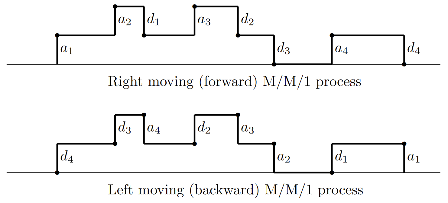
Figure 6.12: FCFS arrivals and departures in right and left moving M/M/1 processes.

We next show how Burke’s theorem can be used to analyze a tandem set of queues. As shown in Figure 6.13, we have an M/M/1 queueing system with Poisson arrivals at rate \(\lambda\) and service at rate \(μ_1\). The departures from this queueing system are the arrivals to a second queueing system, and we assume that a departure from queue 1 at time \(t\) instantaneously enters queueing system 2 at the same time \(t\). The second queueing system has a single server and the service times are IID and exponentially distributed with rate \(μ_2\). The successive service times at system 2 are also independent of the arrivals to systems 1 and 2, and independent of the service times in system 1. Since we have already seen that the departures from the first system are Poisson with rate \(\lambda\) the arrivals to the second queue are Poisson with rate \(\lambda\) Thus the second system is also M/M/1.

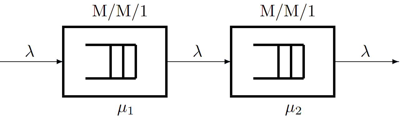
Figure 6.13: A tandem queueing system. Assuming that \(\lambda > \mu_1\) and \(\lambda > \mu_2\), the departures from each queue are Poisson of rate \(\lambda\).

Let \( X(t)\) be the state of queueing system 1 and \(Y (t)\) be the state of queueing system 2. Since \(X(t)\) at time \(t\) is independent of the departures from system 1 prior to \(t\), \(X(t)\) is independent of the arrivals to system 2 prior to time \(t\). Since \(Y (t)\) depends only on the arrivals to system 2 prior to \(t\) and on the service times that have been completed prior to \(t\), we see that \(X(t)\) is independent of \(Y (t)\). This leaves a slight nit-picking question about what happens at the instant of a departure from system 1. We have considered the state \(X(t)\) at the instant of a departure to be the number of customers remaining in system 1 not counting the departing customer. Also the state \(Y (t)\) is the state in system 2 including the new arrival at instant \(t\). The state \(X(t)\) then is independent of the departures up to and including \(t\), so that \(X(t)\) and \(Y (t)\) are still independent.

Next assume that both systems use FCFS service. Consider a customer that leaves system 1 at time \( t\). The time at which that customer arrived at system 1, and thus the waiting time in system 1 for that customer, is independent of the departures prior to \(t\). This means that the state of system 2 immediately before the given customer arrives at time \(t\) is independent of the time the customer spent in system 1. It therefore follows that the time that the customer spends in system 2 is independent of the time spent in system 1. Thus the total system time that a customer spends in both system 1 and system 2 is the sum of two independent random variables.

This same argument can be applied to more than 2 queueing systems in tandem. It can also be applied to more general networks of queues, each with single servers with exponentially distributed service times. The restriction here is that there can not be any cycle of queueing systems where departures from each queue in the cycle can enter the next queue in the cycle. The problem posed by such cycles can be seen easily in the following example of a single queueing system with feedback (see Figure 6.14).

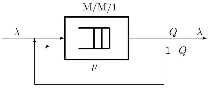
Figure 6.14: A queue with feedback. Assuming that \( μ > \lambda/Q\), the exogenous output is Poisson of rate \(\lambda\).

We assume that the queueing system in Figure 6.14 has a single server with IID exponen­tially distributed service times that are independent of arrival times. The exogenous arrivals from outside the system are Poisson with rate \(\lambda\). With probability \(Q\), the departures from the queue leave the entire system, and, alternatively, with probability \(1 - Q\), they return instantaneously to the input of the queue. Successive choices between leaving the system and returning to the input are IID and independent of exogenous arrivals and of service times. Figure 6.15 shows a sample function of the arrivals and departures in the case in which the service rate \(μ\) is very much greater than the exogenous arrival rate \(\lambda\). Each exogenous arrival spawns a geometrically distributed set of departures and simultaneous re-entries. Thus the overall arrival process to the queue, counting both exogenous arrivals and feedback from the output, is not Poisson. Note, however, that if we look at the Markov process description, the departures that are fed back to the input correspond to self loops from one state to itself. Thus the Markov process is the same as one without the self loops with a service rate equal to \(μQ\). Thus, from Burke’s theorem, the exogenous departures are Poisson with rate \(\lambda\). Also the steady-state distribution of \(X(t)\) is \(P \{X(t) = i\} = (1-\rho ) \rho^i\) where \(\rho=\lambda /(μQ)\) (assuming, of course, that \(\rho< 1\)).

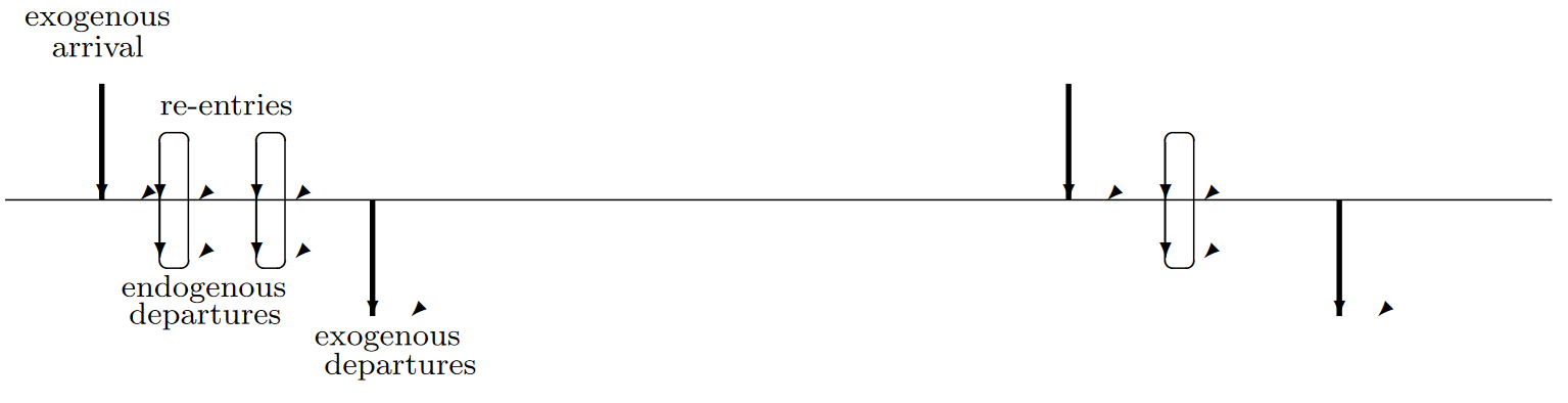
Figure 6.15: Sample path of arrivals and departures for queue with feedback

The tandem queueing system of Figure 6.13 can also be regarded as a combined Markov process in which the state at time \(t\) is the pair \((X(t), Y (t))\). The transitions in this process correspond to, first, exogenous arrivals in which \(X(t)\) increases, second, exogenous departures in which \(Y (t)\) decreases, and third, transfers from system 1 to system 2 in which \(X(t)\) decreases and \(Y (t)\) simultaneously increases. The combined process is not reversible since there is no transition in which \(X(t)\) increases and \(Y (t)\) simultaneously decreases. In the next section, we show how to analyze these combined Markov processes for more general networks of queues.