6.7: Jackson Networks

In many queueing situations, a customer has to wait in a number of different queues before completing the desired transaction and leaving the system. For example, when we go to the registry of motor vehicles to get a driver’s license, we must wait in one queue to have the application processed, in another queue to pay for the license, and in yet a third queue to obtain a photograph for the license. In a multiprocessor computer facility, a job can be queued waiting for service at one processor, then go to wait for another processor, and so forth; frequently the same processor is visited several times before the job is completed. In a data network, packets traverse multiple intermediate nodes; at each node they enter a queue waiting for transmission to other nodes.

Such systems are modeled by a network of queues, and Jackson networks are perhaps the simplest models of such networks. In such a model, we have a network of \(k\) interconnected queueing systems which we call nodes. Each of the \(k\) nodes receives customers (\(i.e.\), tasks or jobs) both from outside the network (exogenous inputs) and from other nodes within the network (endogenous inputs). It is assumed that the exogenous inputs to each node \(i\) form a Poisson process of rate \(r_i\) and that these Poisson processes are independent of each other. For analytical convenience, we regard this as a single Poisson input process of rate \(\lambda_0\), with each input independently going to each node \(i\) with probability \(Q_{0i} =r_i/\lambda_0\).

Each node \(i\) contains a single server, and the successive service times at node \(i\) are IID random variables with an exponentially distributed service time of rate \(μ_i\). The service times at each node are also independent of the service times at all other nodes and independent of the exogenous arrival times at all nodes. When a customer completes service at a given node \(i\), that customer is routed to node \(j\) with probability \(Q_{ij}\) (see Figure 6.16). It is also possible for the customer to depart from the network entirely (called an exogenous departure), and this occurs with probability \(Q_{i0} = 1 -\sum_{j\geq 1} Q_{ij}\). For a customer departing from node \(i\), the next node \(j\) is a random variable with PMF \(\{Q_{ij} , 0 \leq j\leq k\}\).

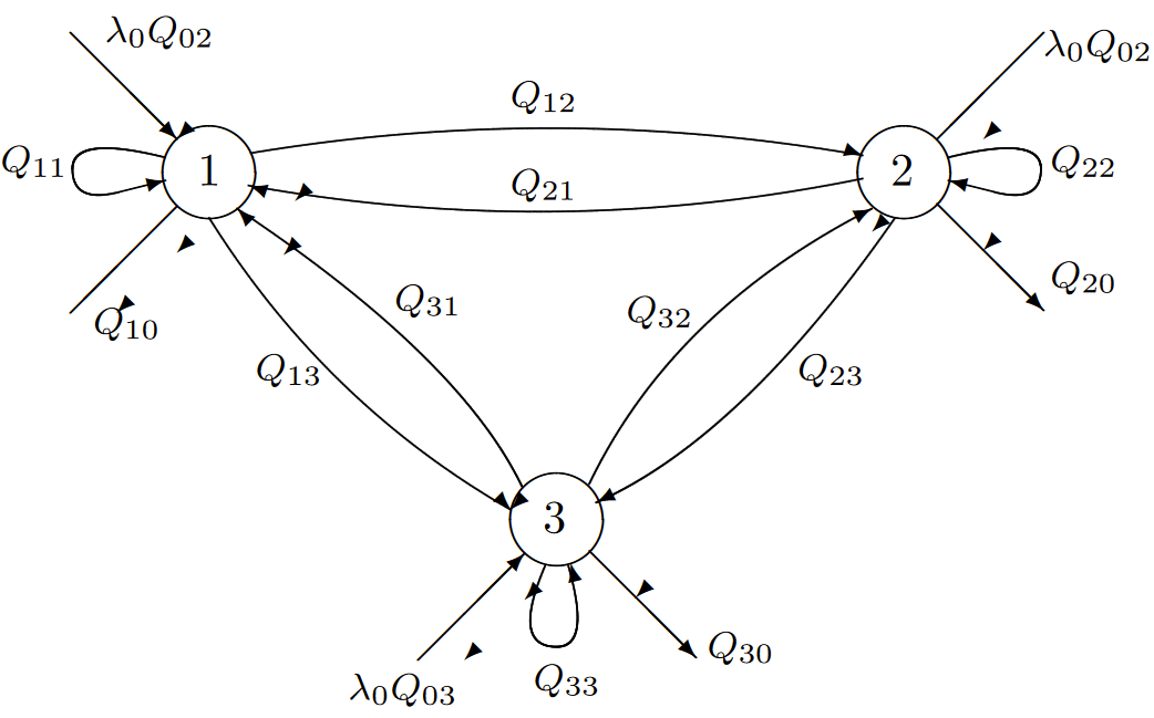
Figure 6.16: A Jackson network with 3 nodes. Given a departure from node \(i\), the probability that departure goes to node \(j\) (or, for \( j = 0\), departs the system) is \(Q_{ij}\). Note that a departure from node \(i\) can re-enter node \(i\) with probability \(Q_{ii}\). The overall exogenous arrival rate is \(\lambda_0\), and, conditional on an arrival, the probability the arrival enters node \(i\) is \(Q_{0i}\).

Successive choices of the next node for customers at node \(i\) are IID, independent of the customer routing at other nodes, independent of all service times, and independent of the exogenous inputs. Notationally, we are regarding the outside world as a fictitious node 0 from which customers appear and to which they disappear.

When a customer is routed from node \(i\) to node \(j\), it is assumed that the routing is instan­taneous; thus at the epoch of a departure from node \(i\), there is a simultaneous endogenous arrival at node \(j\). Thus a node \(j\) receives Poisson exogenous arrivals from outside the system at rate \(\lambda_0 Q_{0j}\) and receives endogenous arrivals from other nodes according to the proba­bilistic rules just described. We can visualize these combined exogenous and endogenous arrivals as being served in FCFS fashion, but it really makes no di↵erence in which order they are served, since the customers are statistically identical and simply give rise to service at node \(j\) at rate \(μ_j\) whenever there are customers to be served.

The Jackson queueing network, as just defined, is fully described by the exogenous input rate the service rates \(\{μ_i\}\), and the routing probabilities \(\{Q_{ij} ; 0 \leq i, j \leq k\}\). The network as a whole is a Markov process in which the state is a vector \(\boldsymbol{m} = (m_1, m_2, . . . , m_k)\), where \(m_i, 1 \leq i \leq k\) is the number of customers at node \(i\). State changes occur upon exogenous arrivals to the various nodes, exogenous departures from the various nodes, and departures from one node that enter another node. In a vanishingly small interval \(\delta\) of time, given that the state at the beginning of that interval is \(\boldsymbol{m}\), an exogenous arrival at node \(j\) occurs in the interval with probability \(\lambda_0Q_{0j}\delta\) and changes the state to \(\boldsymbol{m}' = \boldsymbol{m} +\boldsymbol{e}_j\) where \(\boldsymbol{e}_j\) is a unit vector with a one in position \(j\). If \(m_i > 0\), an exogenous departure from node \(i\) occurs in the interval with probability \( μ_iQ_{i0}\delta\) and changes the state to \(\boldsymbol{m}' = \boldsymbol{m} -\boldsymbol{e}_i+\boldsymbol{e_j}\). Finally, if \(m_i > 0\), a departure from node \(i\) entering node \(j\) occurs in the interval with probability \(μ_iQ_{ij}\delta\) and changes the state to \(\boldsymbol{m}' = \boldsymbol{m} -\boldsymbol{e}_i + \boldsymbol{e}_j \). Thus, the transition rates are given by

\[ \begin{align} q_{\boldsymbol{m,m'}} \quad &= \quad \lambda_0Q_{0j} \qquad \text{for } \boldsymbol{m}' = \boldsymbol{m} + \boldsymbol{e}_j, \quad 1\leq i\leq k \\ &= \quad \mu_iQ_{i0} \qquad \, \text{for }\boldsymbol{m}' = \boldsymbol{m}-\boldsymbol{m_i}, \quad m_i>0, \quad 1\leq i\leq k \\ &= \quad \mu_iQ_{ij} \qquad \, \text{for } \boldsymbol{m}' = \boldsymbol{m} - \boldsymbol{e}_i + \boldsymbol{e}_j, \quad m_i>0, \quad 1\leq i,j\leq, k \\ &= \quad 0 \qquad \qquad \text{for all other choices of }\boldsymbol{m}' \nonumber \end{align} \nonumber \]

Note that a departure from node \(i\) that re-enters node \(i\) causes a transition from state \(\boldsymbol{m}\) back into state \(\boldsymbol{m}\); we disallowed such transitions in sections 6.1 and 6.2, but showed that they caused no problems in our discussion of uniformization. It is convenient to allow these self-transitions here, partly for the added generality and partly to illustrate that the single node network with feedback of Figure 6.14 is an example of a Jackson network.

Our objective is to find the steady-state probabilities \(p(\boldsymbol{m})\) for this type of process, and our plan of attack is in accordance with Theorem 6.6.2; that is, we shall guess a set of transition rates for the backward Markov process, use these to guess \(p(\boldsymbol{m})\), and then verify that the guesses are correct. Before making these guesses, however, we must find out a little more about how the system works, so as to guide the guesswork. Let us define \(\lambda_i\) for each \(i, 1 \leq i \leq k\), as the time-average overall rate of arrivals to node \(i\), including both exogenous and endogenous arrivals. Since \(\lambda_0\) is the rate of exogenous inputs, we can interpret \(\lambda_i/\lambda_0\) as the expected number of visits to node \(i\) per exogenous input. The endogenous arrivals to node \(i\) are not necessarily Poisson, as the example of a single queue with feedback shows, and we are not even sure at this point that such a time-average rate exists in any reasonable sense. However, let us assume for the time being that such rates exist and that the time-average rate of departures from each node equals the time-average rate of arrivals (\(i.e.\), the queue sizes do not grow linearly with time). Then these rates must satisfy the equation

\[ \lambda_j = \sum^k_{j=0} \lambda_iQ_{ij}; \qquad 1\leq j\leq k \nonumber \]

To see this, note that \(\lambda_0Q_{0j}\) is the rate of exogenous arrivals to \(j\). Also \(\lambda_i\) is the time-average rate at which customers depart from queue \(i\), and \(\lambda_iQ_{ij}\) is the rate at which customers go from node \(i\) to node \(j\). Thus, the right hand side of (6.7.4) is the sum of the exogenous and endogenous arrival rates to node \(j\). Note the distinction between the time-average rate of customers going from \(i\) to \(j\) in (6.7.4) and the rate \(q_{\boldsymbol{m,m'}} = μ_iQ_{ij}\) for \(\boldsymbol{m}' = \boldsymbol{m}- \boldsymbol{e}_i+\boldsymbol{e}_j , m_i > 0\) in (6.7.3). The rate in (6.7.3) is conditioned on a state \(\boldsymbol{m}\) with \(m_i > 0\), whereas that in (6.7.4) is the overall time-average rate, averaged over all states.

Note that \(\{Q_{ij} ; 0 \leq i, j \leq k\}\) forms a stochastic matrix and (6.7.4) is formally equivalent to the equations for steady-state probabilities (except that steady-state probabilities sum to 1). The usual equations for steady-state probabilities include an equation for \(j = 0\), but that equation is redundant. Thus we know that, if there is a path between each pair of nodes (including the fictitious node 0), then (6.7.4) has a solution for \(\{\lambda_i; 0\leq i\leq k\}\), and that solution is unique within a scale factor. The known value of \(\lambda_0\) determines this scale factor and makes the solution unique. Note that we don’t have to be careful at this point about whether these rates are time-averages in any nice sense, since this will be verified later; we do have to make sure that (6.7.4) has a solution, however, since it will appear in our solution for \(p(\boldsymbol{m})\). Thus we assume in what follows that a path exists between each pair of nodes, and thus that (6.7.4) has a unique solution as a function of \(\lambda_0\).

We now make the final necessary assumption about the network, which is that \( μ_i >\lambda_i\) for each node \(i\). This will turn out to be required in order to make the process positive recurrent. We also define \(\rho_i\) as \(\lambda_i/\mu_i\). We shall find that, even though the inputs to an individual node \(i\) are not Poisson in general, there is a steady-state distribution for the number of customers at \(i\), and that distribution is the same as that of an M/M/1 queue with the parameter \(\rho_i\).

Now consider the backward time process. We have seen that only three kinds of transitions are possible in the forward process. First, there are transitions from \(\boldsymbol{m}\) to \(\boldsymbol{m}' = \boldsymbol{m} + \boldsymbol{e}_j\) for any \(j, \, 1 \leq j \leq k\). Second, there are transitions from \(\boldsymbol{m}\) to \(\boldsymbol{m}- \boldsymbol{e}_i\) for any \(i, 1 \geq i \leq k\), such that \(m_i > 0\). Third, there are transitions from \(\boldsymbol{m}\) to \(\boldsymbol{m}' = \boldsymbol{m} - \boldsymbol{e}_i + \boldsymbol{e}_j\) for \(1 \leq i, j \leq k\) with \(m_i > 0\). Thus in the backward process, transitions from \(\boldsymbol{m}'\) to \( \boldsymbol{m}\) are possible only for the \(\boldsymbol{m},\, \boldsymbol{m}'\) pairs above. Corresponding to each arrival in the forward process, there is a departure in the backward process; for each forward departure, there is a backward arrival; and for each forward passage from \(i\) to \(j\), there is a backward passage from \(j\) to \( i\).

We now make the conjecture that the backward process is itself a Jackson network with Poisson exogenous arrivals at rates \(\{ \lambda_0Q_{0j}^*\}\), service times that are exponential with rates \(\{μ_i\}\), and routing probabilities \(\{Q_{ij}^*\}\). The backward routing probabilities \(\{ Q_{ij}^* \}\) must be chosen to be consistent with the transition rates in the forward process. Since each transition from \(i\) to \(j\) in the forward process must correspond to a transition from \(j\) to \(i\) in the backward process, we should have

\[ \lambda_i Q_{ij} = \lambda_jQ_{ji}^* \quad ; \quad 0\leq i,j \leq k \nonumber \]

Note that \(\lambda_iQ_{ij}\) represents the rate at which forward transitions go from \(i\) to \(j\), and \(\lambda_i\) rep­resents the rate at which forward transitions leave node \(i\). Equation (6.7.5) takes advantage of the fact that \(\lambda_i\) is also the rate at which forward transitions enter node \(i\), and thus the rate at which backward transitions leave node \(i\). Using the conjecture that the backward time system is a Jackson network with routing probabilities \(\{ Q_{ij}^*; 0 \leq i, j \leq k\}\), we can write down the backward transition rates in the same way as (6.7.1-6.7.3),

\[ \begin{align} q_{\boldsymbol{m,m'}}^* \quad &= \quad \lambda_0Q_{0j}^* \qquad \text{for } \boldsymbol{m}' =\boldsymbol{m}+\boldsymbol{e}_j \\ &= \quad \mu_iQ_{i0}^* \qquad \, \text{for }\boldsymbol{m}' = \boldsymbol{m}- \boldsymbol{e}_i,m_i > 0, 1\leq i\leq k \\ &= \quad \mu_iQ_{ij}^* \qquad \text{for } \boldsymbol{m}'=\boldsymbol{m}-\boldsymbol{e}_i +\boldsymbol{e}_j, \quad m-i>0, \quad 1 \leq i, \quad j\leq k \end{align} \nonumber \]

If we substitute (6.7.5) into (6.7.6)-(6.7.8), we obtain

\[ \begin{align} q_{\boldsymbol{m,m'}}^* \quad &= \quad \lambda_0Q_{j0} \qquad \qquad \text{for } \boldsymbol{m}' =\boldsymbol{m}+\boldsymbol{e}_j, \quad 1\leq j\leq k \\ &= \quad (\mu_i/\lambda_i)\lambda_0Q_{0i} \quad \text{for }\boldsymbol{m}' = \boldsymbol{m}- \boldsymbol{e}_i,m_i > 0, \quad 1\leq i\leq k \\ &= \quad (\mu_i/\lambda_i)\lambda_jQ_{ji} \quad \text{for } \boldsymbol{m}'=\boldsymbol{m}-\boldsymbol{e}_i +\boldsymbol{e}_j, \qquad m_i>0, \quad 1 \leq i, \quad j\leq k \end{align} \nonumber \]

This gives us our hypothesized backward transition rates in terms of the parameters of the original Jackson network. To use theorem 6.6.2, we must verify that there is a set of positive numbers, \(p(\boldsymbol{m})\), satisfying \(\sum_m p(\boldsymbol{m}) = 1\) and \(\sum_m \nu_m p_m < \infty\), and a set of nonnegative numbers \(q_{\boldsymbol{m',m}}^*\) satisfying the following two sets of equations:

\[\begin{align} p(\boldsymbol{m})q_{\boldsymbol{m,m'}} \quad &= \quad p(\boldsymbol{m}')q^*_{\boldsymbol{m',m}} \qquad \text{for all } \boldsymbol{m,m'} \\ \sum_{\boldsymbol{m}}q_{\boldsymbol{m,m'}} \quad &= \quad \sum_{\boldsymbol{m'}} q^*_{\boldsymbol{m,m'}} \qquad \quad \text{for all } \boldsymbol{m}\end{align} \nonumber \]

We verify (6.7.12) by substituting (6.7.1)-(6.7.3) on the left side of (6.7.12) and (6.7.9)-(6.7.11) on the right side. Recalling that \(\rho_i\) is defined as \(\lambda_i/\mu_i\), and cancelling out common terms on each side, we have

\[ \begin{align} p(\boldsymbol{m}) \quad &= \quad p(\boldsymbol{m}')/\rho_j \qquad \text{for } \boldsymbol{m'}=\boldsymbol{m}+\boldsymbol{e}_j \\ p(\boldsymbol{m}) \quad &= \quad p(\boldsymbol{m'})\rho_i \qquad \, \, \, \text{for } \boldsymbol{m'}=\boldsymbol{m}-\boldsymbol{e}_i, m_i >0 \\ p(\boldsymbol{m}) \quad &= \quad p(\boldsymbol{m'})\rho_i/\rho_j \quad \, \, \text{for } \boldsymbol{m'}=\boldsymbol{m}-\boldsymbol{e}_i+\boldsymbol{e}_j, \qquad m_i>0 \end{align} \nonumber \]

Looking at the case \(\boldsymbol{m'} =\boldsymbol{m}-\boldsymbol{e}_i\), and using this equation repeatedly to get from state \((0, 0, . . . , 0)\) up to an arbitrary \(\boldsymbol{m}\), we obtain

\[ p(\boldsymbol{m}) = p(0,0,...,0) \prod^k_{i=1} \rho^{m_i}_i \nonumber \]

It is easy to verify that (6.7.17) satisfies (6.7.14)-(6.7.16) for all possible transitions. Summing over all \(\boldsymbol{m}\) to solve for \(p(0, 0, . . . , 0)\), we get

\[ \begin{aligned} 1 \quad = \quad \sum_{m_1,m_2,...,m_k} p(\boldsymbol{m}) \quad &= \quad p(0,0,...,0) \sum_{m_1}\rho_1^{m_1}\sum_{m_2}\rho_2^{m_2}...\sum_{m_k}\rho_k^{m_k} \\ &= \quad p(0,0...,0)(1-\rho_1)^{-1}(1-\rho_2)^{-1}...(1-\rho_k)^{-1} \end{aligned} \nonumber \]

Thus, \(p(0,0,...,0) = (1-p_1)(1-p_2)...(1-p_k)\), and substituting this in (6.7.17), we get

\[ p(\boldsymbol{m})=\prod^k_{i=1} p_i(m_i) = \prod^k_{i=1} \left[ (1-\rho_i)\rho_i^{m_i} \right] \nonumber \]

where \(p_i(m)=(1-\rho_i)\rho^m_i\) is the steady-state distribution of a single M/M/1 queue. Now i that we have found the steady-state distribution implied by our assumption about the backward process being a Jackson network, our remaining task is to verify (6.7.13)

To verify (6.7.13), \(i.e.\), \(\sum_{\boldsymbol{m'}} q_{\boldsymbol{m,m'}} = \sum_{\boldsymbol{m'}} q^*_{\boldsymbol{m,m'}} \), first consider the right side. Using (6.7.6) to sum over all \(\boldsymbol{m}' = \boldsymbol{m} + \boldsymbol{e}_j \), then (6.7.7) to sum over \(\boldsymbol{m}' = \boldsymbol{m} - \boldsymbol{e}_i\) (for \(i\) such that \(m_i>0\)), and finally (6.7.8) to sum over \(\boldsymbol{m}' = \boldsymbol{m} - \boldsymbol{e}_i+\boldsymbol{e}_j\), (again for \(i\) such that \(m_i > 0\)), we get

\[ \sum_{\boldsymbol{m'}} q^*_{\boldsymbol{m,m'}} = \sum^k_{j=1}\lambda_0Q_{0j}^*+\sum_{i:m_j>0} \mu_iQ_{i0}^* + \sum_{i:m_j>0} \mu_i \sum^k_{j=1} Q_{ij}^* \nonumber \]

Using the fact \(Q^*\) is a stochastic matrix, then,

\[ \sum_{\boldsymbol{m'}} q^*_{\boldsymbol{m,m'}} = \lambda_0+\sum_{i:m_i>0} \mu_i \nonumber \]

The left hand side of (6.7.13) can be summed in the same way to get the result on the right side of (6.7.20), but we can see that this must be the result by simply observing that \(\lambda_0\) is the rate of exogenous arrivals and \(\sum_{i:m_i>0} μ_i\) is the overall rate of service completions in state \(\boldsymbol{m}\). Note that this also verifies that \(\nu_{\boldsymbol{m}} = \sum_{\boldsymbol{m'}} q_{\boldsymbol{m,m'}} \geq \lambda_0 + \sum_i μ_i\), and since \(\nu_{\boldsymbol{m}}\) is bounded, \(\sum_{\boldsymbol{m}} \nu_{\boldsymbol{m}} p(\boldsymbol{m}) < \infty\). Since all the conditions of Theorem 6.6.2 are satisfied, \(p(\boldsymbol{m})\), as given in (6.7.18), gives the steady-state probabilities for the Jackson network. This also verifies that the backward process is a Jackson network, and hence the exogenous departures are Poisson and independent.

Although the exogenous arrivals and departures in a Jackson network are Poisson, the endogenous processes of customers traveling from one node to another are typically not Poisson if there are feedback paths in the network. Also, although (6.7.18) shows that the numbers of customers at the different nodes are independent random variables at any given time in steady-state, it is not generally true that the number of customers at one node at one time is independent of the number of customers at another node at another time.

There are many generalizations of the reversibility arguments used above, and many network situations in which the nodes have independent states at a common time. We discuss just two of them here and refer to Kelly, [13], for a complete treatment.

For the first generalization, assume that the service time at each node depends on the number of customers at that node, \(i.e.\), \(μ_i\) is replaced by \(μ_{i,m_i}\). Note that this includes the M/M/m type of situation in which each node has several independent exponential servers. With this modification, the transition rates in (6.7.2) and (6.7.3) are modified by replacing \(μ_i\) with \(μ_{i,m_i}\). The hypothesized backward transition rates are modified in the same way, and the only effect of these changes is to replace \(\rho_i\) and \(\rho_j\) for each \(i\) and \(j\) in (6.7.14)-(6.7.16) with \(\rho_{i,m_i} =\lambda_i/\mu_{i,m_i}\) and \(\rho_{j,m_j} = \lambda_j/\mu_{j,m_j}\). With this change, (6.7.17) becomes

\[ \begin{align} p(\boldsymbol{m}) \quad &= \quad \prod^k_{i=1} p_i (m_i) \quad = \quad \prod^k_{i=1} p_i \ref{0} \prod^{m_i}_{j=0} \rho_{i,j} \\ p_i(0) \quad &= \quad \left[ 1+ \sum^{\infty}_{m=1} \prod^{m-1}_{j=0} \rho_{i,j} \right]^{-1} \end{align} \nonumber \]

Thus, \(p(\boldsymbol{m})\) is given by the product distribution of \(k\) individual birth-death systems.

Closed Jackson networks

The second generalization is to a network of queues with a fixed number \(M\) of customers in the system and with no exogenous inputs or outputs. Such networks are called closed Jackson networks, whereas the networks analyzed above are often called open Jackson networks. Suppose a \(k\) node closed network has routing probabilities \(Q_{ij} ,\, 1 \leq i, j \leq k\), where \(\sum_j Q_{ij} = 1\), and has exponential service times of rate \(μ_i\) (this can be generalized to \(μ_{i,m_i\) as above). We make the same assumptions as before about independence of service variables and routing variables, and assume that there is a path between each pair of nodes. Since \(\{ Q_{ij} ; 1 \leq i, j \leq k\}\) forms an irreducible stochastic matrix, there is a one dimensional set of solutions to the steady-state equations

\[ \lambda_j = \sum_i \lambda_iQ_{ij}; \qquad 1\leq j \leq k \nonumber \]

We interpret \(\lambda_i \) as the time-average rate of transitions that go into node \(i\). Since this set of equations can only be solved within an unknown multiplicative constant, and since this constant can only be determined at the end of the argument, we define \(\{\pi_i; 1 \leq i \leq k\}\) as the particular solution of (6.7.23) satisfying

\[ \pi_j = \sum_i \pi_i Q_{ij}; 1\leq j \leq k ; \sum_i \pi_i =1 \nonumber \]

Thus, for all \(i, \, \lambda_i= \alpha\pi_i\), where \(\alpha\) is some unknown constant. The state of the Markov process is again taken as \(\boldsymbol{m} = (m_1, m_2, . . . , m_k)\) with the condition \(\sum_i m_i = M\). The transition rates of the Markov process are the same as for open networks, except that there are no exogenous arrivals or departures; thus (6.7.1)-(6.7.3) are replaced by

\[ q_{\boldsymbol{m,m'}} = \mu_i q_{ij} \quad \text{for } \boldsymbol{m'} = \boldsymbol{m} - \boldsymbol{e_i} + \boldsymbol{e_j}, \quad m_i>0, \, \, \, 1\leq i,j \leq k \nonumber \]

We hypothesize that the backward time process is also a closed Jackson network, and as before, we conclude that if the hypothesis is true, the backward transition rates should be

\[ \begin{align} q^*_{\boldsymbol{m,m'}} \quad &= \quad \mu_iQ^*_{ij} \quad \text{for } \boldsymbol{m'=m-e_i+e_j}, \, m_i>0, \, 1\leq i,j\leq k \\ \text{where } \lambda_iQ_{ij} \quad &= \quad \lambda_jQ^*_{ji} \quad \text{for } 1\leq i,j \leq k \end{align} \nonumber \]

In order to use Theorem 6.6.2 again, we must verify that a PMF \(p(\boldsymbol{m})\) exists satisfying \(p(\boldsymbol{m})q_{\boldsymbol{m,m'}} = p(\boldsymbol{m'})q^*_{\boldsymbol{m',m}}\) for all possible states and transitions, and we must also verify that \(\sum_{\boldsymbol{m'}} q_{\boldsymbol{m,m'}} = \sum_{\boldsymbol{m'}}q^*_{\boldsymbol{m,m'}}\) for all possible \(\boldsymbol{m}\). This latter verification is virtually the same as before and is left as an exercise. The former verification, with the use of (72), (73), and (74), becomes

\[ p(\boldsymbol{m})(\mu_i/\lambda_i) = p(\boldsymbol{m'})(\mu_j)/\lambda_j) \quad \text{for } \boldsymbol{m'=m-e_i+e_j}, \quad m_i>0 \nonumber \]

Using the open network solution to guide our intuition, we see that the following choice of \(p(\boldsymbol{m})\) satisfies (6.7.28) for all possible \(\boldsymbol{m}\) (\(i.e.\), all \(\boldsymbol{m}\) such that \(\sum_i m_i = M \))

\[ p(\boldsymbol{m}) = A \prod^k_{i=1} (\lambda_i/\mu_i)^{m_i}; \quad \text{for }\boldsymbol{m}\text{ such that } \sum_i m_i =M \nonumber \]

The constant \(A\) is a normalizing constant, chosen to make \(p(\boldsymbol{m})\) sum to unity. The problem with (6.7.29) is that we do not know \(\lambda_i\) (except within a multiplicative constant independent of \(i\)). Fortunately, however, if we substitute \(\pi_i/\alpha\) for \(\lambda_i\) we see that \(\alpha\) is raised to the power \(- M \), independent of the state \(\boldsymbol{m}\). Thus, letting \(A'= A\alpha - M\), our solution becomes

\[ \begin{align} p(\boldsymbol{m}) \quad &= \quad A'\prod^K_{i=1} ( \pi_i/\mu_i)^{m_i}: \,\,\, \text{for }\boldsymbol{m}\text{ such that } \sum_i m_i=M \\ \dfrac{1}{A'} \quad &= \quad \left. \sum_{\boldsymbol{m}: \sum_im_i=M} \prod^k_{i=1} \dfrac{\pi_i}{\mu_i} \right)^{m_i} \end{align} \nonumber \]

Note that the steady-state distribution of the closed Jackson network has been found with­ out solving for the time-average transition rates. Note also that the steady-state distribution looks very similar to that for an open network; that is, it is a product distribution over the nodes with a geometric type distribution within each node. This is somewhat misleading, however, since the constant \(A'\) can be quite difficult to calculate. It is surprising at first that the parameter of the geometric distribution can be changed by a constant multiplier in (6.7.30) and (6.7.31) (\(i.e.\), \(\pi_i\) could be replaced with \(\lambda_i\)) and the solution does not change; the important quantity is the relative values of \(\pi_i/μ_i\) from one value of \(i\) to another rather than the absolute value

In order to find \(\lambda_i\) (and this is important, since it says how quickly the system is doing its work), note that \(\lambda_i = \mu_i\text{Pr}\{m_i>0\}\). Solving for \(\text{Pr}\{ m_i > 0\}\) requires finding the constant \(A'\) in (6.7.25). In fact, the major difference between open and closed networks is that the relevant constants for closed networks are tedious to calculate (even by computer) for large networks and large \(M \).