6.8: Semi-Markov Processes

Semi-Markov processes are generalizations of Markov processes in which the time intervals between transitions have an arbitrary distribution rather than an exponential distribution. To be specific, there is an embedded Markov chain, \(\{X_n; n \geq 0\}\) with a finite or count­ably infinite state space, and a sequence \(\{U_n; n \geq 1 \}\) of holding intervals between state transitions. The epochs at which state transitions occur are then given, for \(n \geq 1\), as \(S_n = \sum_{m=1}^n U_n\). The process starts at time 0 with \(S_0\) defined to be 0. The semi-Markov process is then the continuous-time process \(\{X(t); t \geq 0\}\) where, for each \(n \geq 0\), \(X(t) = X_n\) for \(t\) in the interval \(S_n \leq X_n < S_{n+1}\). Initially, \(X_0 = i\) where \(i\) is any given element of the state space.

The holding intervals \(\{U_n; n \geq 1\}\) are nonnegative rv’s that depend only on the current state \(X_{n-1}\) and the next state \(X_n\). More precisely, given \(X_{n-1} = j\) and \(X_n = k\), say, the interval \(U_n\) is independent of \(\{U_m; m < n\}\) and independent of \(\{X_m; m < n - 1\}\) The conditional distribution function for such an interval \(U_n\) is denoted by \(G_{ij} (u)\), \(i.e.\),

\[ \text{Pr} \{ U_n\leq u | X_{n-1} = j,X_n = k \} = G_{jk} \ref{u} \nonumber \]

The dependencies between the rv’s \(\{X_n; n \geq 0\}\) and \(\{U_n; n \geq 1\}\) is illustrated in Figure 6.17.

The conditional mean of \(U_n\), conditional on \(X_{n-1} = j,\, X_n = k\), is denoted \(\overline{U} (j, k)\), \(i.e.\),

\[ \overline{U}(i,j) = \mathsf{E} [U_n | X_{n-1} =i ,X_n=j] = \int_{u\geq 0} [1-G_{ij}(u)] du \nonumber \]

A semi-Markov process evolves in essentially the same way as a Markov process. Given an initial state, \(X_0 = i\) at time 0, a new state \(X_1 = j\) is selected according to the embedded chain with probability \(P_{ij}\). Then \(U_1 = S_1\) is selected using the distribution \(G_{ij} (u)\). Next a new state \(X_2 = k\) is chosen according to the probability \(P_{jk}\); then, given \(X_1 = j\) and \(X_2 = k\), the interval \(U_2\) is selected with distribution function \(G_{jk}(u)\). Successive state transitions and transition times are chosen in the same way.

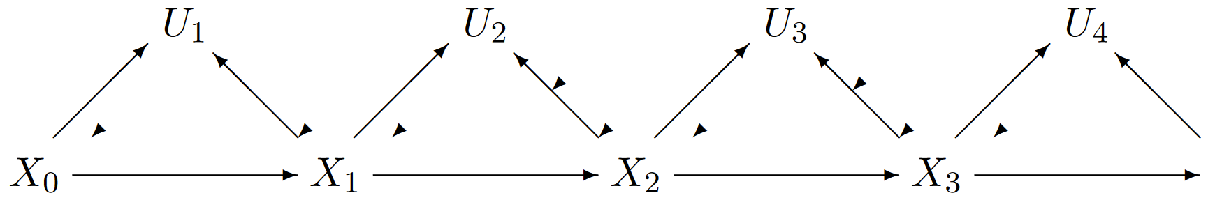
Figure 6.17: The statistical dependencies between the rv’s of a semi-Markov process. Each holding interval \(U_n\), conditional on the current state \(X_{n-1}\) and next state \(X_n\), is independent of all other states and holding intervals. Note that, conditional on \(X_n\), the holding intervals \(U_n, U_{n-1} , . . . ,\) are statistically independent of \(U_{n+1}, X_{n+2}, . . .\).

The steady-state behavior of semi-Markov processes can be analyzed in virtually the same way as Markov processes. We outline this in what follows, and often omit proofs where they are the same as the corresponding proof for Markov processes. First, since the holding intervals, \(U_n\), are rv’s, the transition epochs, \(S_n = \sum^n_{m=1} U_n\), are also rv’s. The following lemma then follows in the same way as Lemma 6.2.1 for Markov processes.

Lemma 6.8.1. Let \(M_i(t)\) be the number of transitions in a semi-Markov process in the interval \((0, t]\) for some given initial state \(X_0 = i\). Then \(\lim_{t\rightarrow\infty} M_i(t) = \infty\) WP1.

In what follows, we assume that the embedded Markov chain is irreducible and positive-recurrent. We want to find the limiting fraction of time that the process spends in any given state, say \(j\). We will find that this limit exists WP1, and will find that it depends only on the steady-state probabilities of the embedded Markov chain and on the expected holding interval in each state. This is given by

\[ \overline{U}(j) = \mathsf{E}[U_n | X_{n-1} =j] = \sum_k P_{jk}\mathsf{E}[U_n|X_{n-1}=j,X_n=k] = \sum_k P_{jk}\overline{U} (j,k) \nonumber \]

where \(\overline{U} (j, k)\) is given in 6.87. The steady-state probabilities \(\{\pi_i; i \geq 0\}\) for the embedded chain tell us the fraction of transitions that enter any given state \(i\). Since \(\overline{U} (i)\) is the expected holding interval in \(i\) per transition into \(i\), we would guess that the fraction of time spent in state \(i\) should be proportional to \(\pi_i\overline{U} (i)\). Normalizing, we would guess that the time-average probability of being in state \(i\) should be

\[ p_j = \dfrac{\pi_j \overline{U} (j)}{\sum_k \pi_k\overline{U} (k)} \nonumber \]

Identifying the mean holding interval, \(\overline{U}_j\) with \(1/\nu_j\), this is the same result that we estab­lished for the Markov process case. Using the same arguments, we find this is valid for the semi-Markov case. It is valid both in the conventional case where each \(p_j\) is positive and \(\sum_j p_j = 1\), and also in the case where \(\sum_k \pi_k\overline{U} \ref{k} = \infty\), where each \(p_j = 0\). The analysis is based on the fact that successive transitions to some given state, say \(j\), given \(X_0 = i\), form a delayed renewal process.

Lemma 6.8.2. Consider a semi-Markov process with an irreducible recurrent embedded chain \(\{X_n; n \geq 0\}\). Given \(X_0 = i\), let \(\{M_{ij} (t); t \geq 0\}\) be the number of transitions into a given state \(j\) in the interval \((0, t]\). Then \(\{M_{ij} (t); t \geq 0\}\) is a delayed renewal process (or, if \(j = i\), is an ordinary renewal process).

This is the same as Lemma 6.2.2, but it is not quite so obvious that successive intervals be­tween visits to state \(j\) are statistically independent. This can be seen, however, from Figure 6.17, which makes it clear that, given \(X_n = j\), the future holding intervals, \(U_n, U_{n+1}, . . . ,\) are independent of the past intervals \(U_{n-1}, U_{n-2},...\).

Next, using the same renewal reward process as in Lemma 6.2.3, assigning reward 1 when­ever \(X(t) = j\), we define \(W_n\) as the interval between the \(n- 1\)st and the \(n\)th entry to state \(j\) and get the following lemma:

Lemma 6.8.3. Consider a semi-Markov process with an irreducible, recurrent, embedded Markov chain starting in \(X_0 = i\). Then with probability 1, the limiting time-average in state \(j\) is given by \(p_j \ref{i} =\frac{\overline{U}_j}{\overline{W}(j)}\).

This lemma has omitted any assertion about the limiting ensemble probability of state \(j\), \(i.e.\), \(\lim_{t\rightarrow \infty} \text{Pr}\{ X(t) = j\}\). This follows easily from Blackwell’s theorem, but depends on whether the successive entries to state \(j\), \(i.e.\), \(\{W_n; n \geq 1\}\), are arithmetic or non-arithmetic. This is explored in Exercise 6.33. The lemma shows (as expected) that the limiting time-average in each state is independent of the starting state, so we henceforth replace \(p_j (i)\) with \(p_j\).

Next, let \(M_i(t)\) be the total number of transitions in the semi-Markov process up to and including time \(n\), given \(X_0 = i\). This is not a renewal counting process, but, as with Markov processes, it provides a way to combine the time-average results for all states \(j\). The following theorem is the same as that for Markov processes, except for the omission of ensemble average results.

Theorem 6.8.1. Consider a semi Markov process with an irreducible, positive-recurrent, embedded Markov chain. Let \(\{\pi_j ; j \geq 0\}\) be the steady-state probabilities of the embedded chain and let \(X_0 = i\) be the starting state. Then, with probability 1, the limiting time-average fraction of time spent in any arbitrary state \(j\) is given by

\[ p_j = \dfrac{\pi_j\overline{U}(j)}{\sum_k\pi_k \overline{U} (j)} \nonumber \]

The expected time between returns to state \(j\) is

\[ \overline{W}(j) = \dfrac{\sum_k \pi_k \overline{U}(k)}{\pi_j} \nonumber \]

and the rate at which transitions take place is independent of \(X_0\) and given by

\[ \lim_{t\rightarrow \infty} \dfrac{M_i(t)}{t} = \dfrac{1}{\sum_k\pi_k \overline{U}(k)} \quad \text{WP1} \nonumber \]

For a semi-Markov process, knowing the steady state probability of \(X(t) = j\) for large \(t\) does not completely specify the steady-state behavior. Another important steady state question is to determine the fraction of time involved in \(i\) to \(j\) transitions. To make this notion precise, define \(Y (t)\) as the residual time until the next transition after time \(t\) (\(i e.\), \(t + Y (t)\) is the epoch of the next transition after time \(t\)). We want to determine the fraction of time \(t\) over which \(X(t) = i\) and \(X(t + Y (t)) = j\). Equivalently, for a non-arithmetic process, we want to determine \(\text{Pr}\{ X(t) = i,\, X(t + Y \ref{t} = j)\}\) in the limit as \(t \rightarrow \infty\). Call this limit \(Q(i, j)\).

Consider a renewal process, starting in state \(i\) and with renewals on transitions to state \(i\). Define a reward \(R(t) = 1\) for \(X(t) = i\), \(X(t + Y (t)) = j\) and \(R(t) = 0\) otherwise (see Figure 6.18). That is, for each \(n\) such that \(X(S_n) = i\) and \(X(S_{n+1}) = j\), \(R(t) = 1\) for \(S_n \leq t < S_{n+1}\). The expected reward in an inter-renewal interval is then \(P_{ij} \overline{U} (i, j)\). It follows that \(Q(i, j)\) is given by

\[Q(i,j) = \lim_{t\rightarrow \infty} \dfrac{\int^t_0 R(\tau) d\tau}{t} = \dfrac{P_{ij}\overline{U}(i,j)}{\overline{W}(i)} = \dfrac{p_iP_{ij}\overline{U}(i,j)}{\overline{U}(i) } \nonumber \]

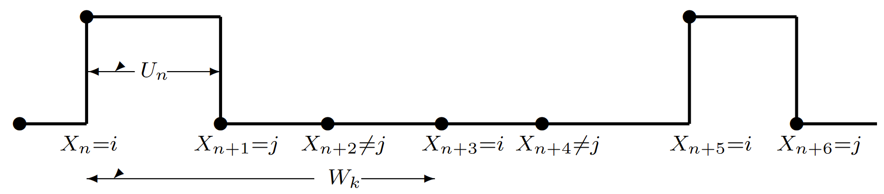
Figure 6.18: The renewal-reward process for \(i\) to \(j\) transitions. The expected value of \(U_n\) if \(X_n = i\) and \(X_{n+1} = j\) is \(\overline{U} (i, j)\) and the expected interval between entries to \(i\) is \(\overline{W} (i)\).

Example — the M/G/1 queue

As one example of a semi-Markov chain, consider an M/G/1 queue. Rather than the usual interpretation in which the state of the system is the number of customers in the system, we view the state of the system as changing only at departure times; the new state at a departure time is the number of customers left behind by the departure. This state then remains fixed until the next departure. New customers still enter the system according to the Poisson arrival process, but these new customers are not considered as part of the state until the next departure time. The number of customers in the system at arrival epochs does not in general constitute a “state” for the system, since the age of the current service is also necessary as part of the statistical characterization of the process.

One purpose of this example is to illustrate that it is often more convenient to visualize the transition interval \(U_n = S_n - S_{n-1}\) as being chosen first and the new state \(X_n\) as being chosen second rather than choosing the state first and the transition time second. For the M/G/1 queue, first suppose that the state is some \(i > 0\). In this case, service begins on the next customer immediately after the old customer departs. Thus, \(U_n\), conditional on \(X_n = i\) for \(i > 0\), has the distribution of the service time, say \(G(u)\). The mean interval until a state transition occurs is

\[ \overline{U}(i) = \int^{\int}_0 [1-G(u)]du; \quad i>0 \nonumber \]

Given the interval \(u\) for a transition from state \(i > 0\), the number of arrivals in that period is a Poisson random variable with mean \(\lambda u\), where \(\lambda\) is the Poisson arrival rate. Since the next state \(j\) is the old state \(i\), plus the number of new arrivals, minus the single departure,

\[\text{Pr} \{ X_{n+1}=j|X_n =i,U_n=u\} = \dfrac{(\lambda u)^{j+i+1}\exp (-\lambda u)}{(j-i+1)!} \nonumber \]

for \(j \geq i-1\). For \(j < i -1\), the probability above is 0. The unconditional probability \(P_{ij}\) of a transition from \(i\) to \(j\) can then be found by multiplying the right side of \ref{6.95} by the probability density \(g(u)\) of the service time and integrating over \(u\).

\[ P_{ij} = \int^{\infty}_0 \dfrac{G(u)(\lambda u)^{j-i+1}\exp (-\lambda u)}{(j-i+1)} du; \quad j \geq i-1, i>0 \nonumber \]

For the case \(i = 0\), the server must wait until the next arrival before starting service. Thus the expected time from entering the empty state until a service completion is

\[ \overline{U} \ref{0} = (1/\lambda ) + \int^{\infty}_0 [1-G(u)]du \nonumber \]

We can evaluate \(P_{0j}\) by observing that the departure of that first arrival leaves \(j\) customers in this system if and only if \(j\) customers arrive during the service time of that first customer; \(i.e.\), the new state doesn’t depend on how long the server waits for a new customer to serve, but only on the arrivals while that customer is being served. Letting \(g(u)\) be the density of the service time,

\[ P_{0j} = \int^{\infty}_0 \dfrac{g(u)(\lambda u)^j \exp (-\lambda u)}{j!} du; \quad j\geq 0 \nonumber \]