
7.7: Submartingales and Supermartingales
- Page ID
- 76993

Submartingales and supermartingales are simple generalizations of martingales that provide many useful results for very little additional work. We will subsequently derive the Kolmogorov submartingale inequality, which is a powerful generalization of the Markov inequality. We use this both to give a simple proof of the strong law of large numbers and also to better understand threshold crossing problems for random walks.
Definition 7.7.1. A submartingale is an integer-time stochastic process {\(Z_n; n ≥ 1\)} that satisfies the relations
\[ \mathsf{E} [|Z_n|]<\infty \quad ; \quad \mathsf{E}[Z_n|Z_{n-1},Z_{n-2},...,Z_1] \geq Z_{n-1} \quad ; \quad n \geq 1 \nonumber \]
A supermartingale is an integer-time stochastic process {\(Z_n; n ≥ 1\)} that satisfies the relations
\[ \mathsf{E}[|Z_n|] <\infty \quad ; \quad \mathsf{E}[Z_n|Z_{n-1},Z_{n-1},...,Z_1]\leq Z_{n-1} \quad ; \quad n \geq 1 \nonumber \]
In terms of our gambling analogy, a submartingale corresponds to a game that is at least fair, \(i.e.\), where the expected fortune of the gambler either increases or remains the same. A supermartingale is a process with the opposite type of inequality.1
Since a martingale satisfies both (7.7.1) and (7.7.2) with equality, a martingale is both a submartingale and a supermartingale. Note that if {\(Z_n; n ≥ 1\)} is a submartingale, then {\(−Z_n; n ≥ 1\)} is a supermartingale, and conversely. Thus, some of the results to follow are stated only for submartingales, with the understanding that they can be applied to supermartingales by changing signs as above.
Lemma 7.6.1, with the equality replaced by inequality, also applies to submartingales and supermartingales. That is, if {\(Z_n; n ≥ 1\)} is a submartingale, then
\[ \mathsf{E}[Z_n|Z_i,Z_{i-1},...,Z_1] \geq Z_i \quad ; \quad 1\leq i<n \nonumber \]
and if {\(Z_n; n ≥ 1\)} is a supermartingale, then
\[ \mathsf{E}[Z_n|Z_i,Z_{i-1},...,Z_1] \leq Z_i \quad ; \quad 1 \leq i<n \nonumber \]
Equations (7.7.3) and (7.7.4) are verified in the same way as Lemma 7.6.1 (see Exercise 7.18). Similarly, the appropriate generalization of (7.6.13) is that if {\(Z_n; n ≥ 1\)} is a submartingale, then
\[ \mathsf{E}[Z_n] \geq \mathsf{E}[Z_i] \quad ; \quad \text{for all } i, \, 1\leq i <n \nonumber \]
and if {\(Z_n; n ≥ 1\)} is a supermartingale, then
\[ \mathsf{E}[Z_n] \leq \mathsf{E}[Z_i] \quad ; \quad \text{for all } i, \, 1 \leq i<n \nonumber \]
A random walk {\(S_n; n ≥ 1\)} with \(S_n = X_1 +... + X_n\) is a submartingale, martingale, or supermartingale respectively for \(\overline{X} ≥ 0, \overline{X} = 0\), or \(\overline{X} ≤ 0\). Also, if \(X\) has a semi-invariant moment generating function \(\gamma (r)\) for some given \(r\), and if \(Z_n\) is defined as \(Z_n = \exp (rS_n)\), then the process {\(Z_n; n ≥ 1\)} is a submartingale, martingale, or supermartingale respectively for \(\gamma \ref{r} ≥ 0,\, \gamma \ref{r} = 0\), or \( \gamma \ref{r} ≤ 0\). The next example gives an important way in which martingales and submartingales are related.
Example 7.7.1 (Convex functions of martingales) Figure 7.11 illustrates the graph of a convex function \(h\) of a real variable \(x\). A function \(h\) of a real variable is defined to be convex if, for each point \(x_1\), there is a real number \(c\) with the property that \(h(x_1) + c(x − x_1) ≤ h(x)\) for all \(x\)
Geometrically, this says that every tangent to \( h(x)\) lies on or below \(h(x)\). If \( h(x)\) has a derivative at \(x_1\), then \(c\) is the value of that derivative and \(h(x_1) + c(x − x_1)\) is the tangent line at \(x_1\). If \(h(x)\) has a discontinuous slope at \(x_1\), then there might be many choices for \(c\); for example, \(h(x) = |x|\) is convex, and for \(x_1 = 0\), one could choose any \(c\) in the range −1 to +1.
A simple condition that implies convexity is a nonnegative second derivative everywhere. This is not necessary, however, and functions can be convex even when the first derivative does not exist everywhere. For example, the function \(\gamma (r)\) in Figure 7.8 is convex even though it it is finite at \(r = r_+\) and infinite for all \(r > r_+\).
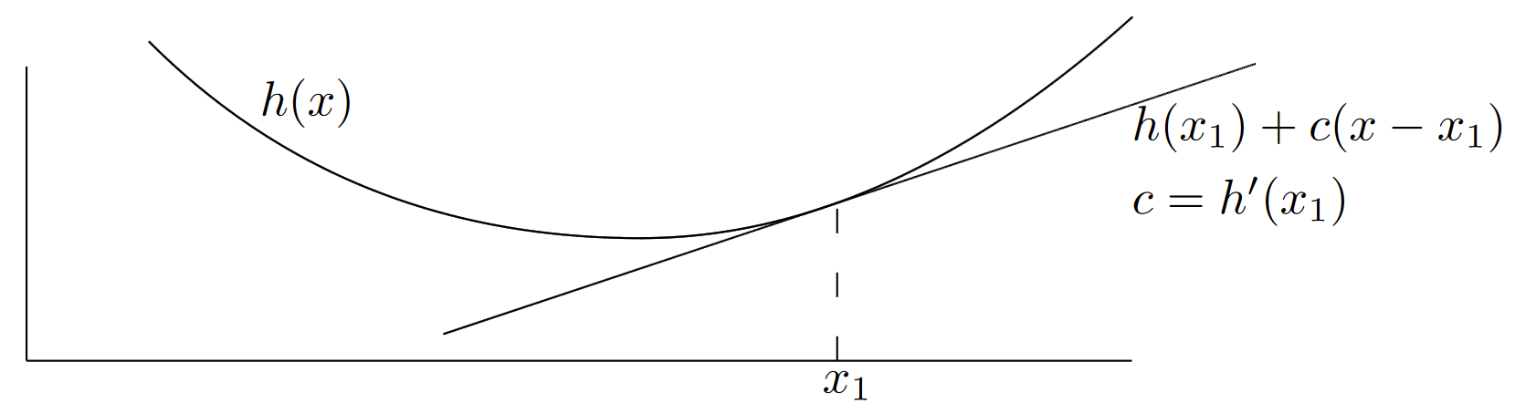
| Figure 7.11: Convex functions: For each \(x_1\), there is a value of \(c\) such that, for all \(x\), \(h(x_1) + c(x − x_1) ≤ h(x)\). If \(h\) is differentiable at \(x_1\), then \(c\) is the derivative of \(h\) at \(x_1\) |
Jensen’s inequality states that if \(h\) is convex and \(X\) is a random variable with an expectation, then \(h(\mathsf{E} [X]) ≤ \mathsf{E} [h(X)]\). To prove this, let \(x_1 = \mathsf{E} [X]\) and choose \(c\) so that \(h(x_1) + c(x − x_1) ≤ h(x)\). Using the random variable \(X\) in place of \(x\) and taking expected values of both sides, we get Jensen’s inequality. Note that for any particular event \(A\), this same argument applies to \(X\) conditional on \(A\), so that \(h(\mathsf{E} [X | A]) ≤ \mathsf{E} [h(X) | A]\). Jensen’s inequality is very widely used; it is a minor miracle that we have not required it previously.
Theorem 7.7.1. Assume that \(h\) is a convex function of a real variable, that {\(Z_n; n ≥ 1\)} is a martingale or submartingale, and that \(\mathsf{E} [|h(Z_n)|] < \infty \) for all \(n\). Then {\(h(Z_n); n ≥ 1\)} is a submartingale.
Proof: For any choice of \(z_1, . . . , z_{n−1}\), we can use Jensen’s inequality with the conditioning probabilities to get
\[\mathsf{E}[h(Z_n)|Z_{n-1}=z_{n-1},...,Z_1=z_1] \geq h(\mathsf{E}[Z_n|Z_{n-1}=z_{n-1},...,Z_1=z_1])=h(z_{n-1}) \nonumber \]
For any choice of numbers \(h_1, . . . , h_{n−1}\) in the range of the function \(h\), let \(z_1, . . . , z_{n−1}\) be arbitrary numbers satisfying \(h(z_1)=h_1, . . . , h(z_{n−1})=h_{n−1}\). For each such choice, (7.7.7) holds, so that
\[ \begin{align} \mathsf{E}[h(Z_n)|h(Z_{n-1})=h_{n-1},...,h(Z_1)=h_1] \quad &\geq \quad h(\mathsf{E}[Z_n|h(Z_{n-1})=h_{n-1},...,h(Z_1)=h_1]) \nonumber \\ &= \quad h(z_{n-1}) = h_{n-1} \end{align} \nonumber \]
completing the proof.
\( \square \)
Some examples of this result, applied to a martingale {\(Z_n; n ≥ 1\)}, are as follows:
\[ \begin{align} &\{ |Z_n|;\, n\geq \} \text{ is a submartingale} \\ &\{ Z_n^2; \, n\geq 1\} \text{ is a submartingale if } \mathsf{E}[Z_n^2]<\infty \\ &\{\exp (rZ_n); \, n\geq 1\} \text{ is a submartingale for } r \text{ such that } \mathsf{E}[\exp (rZ_n)]<\infty \end{align} \nonumber \]
A function of a real variable \(h(x)\) is defined to be concave if \(−h(x)\) is convex. It then follows from Theorem 7.7.1 that if \(h\) is concave and {\(Z_n; n ≥ 1\)} is a martingale, then {\(h(Z_n); n ≥ 1\)} is a supermartingale (assuming that \(\mathsf{E} [|h(Z_n)|] < \infty \)). For example, if {\(Z_n; n ≥ 1\)} is a positive martingale and \(\mathsf{E} [| \ln (Z_n)|] < \infty \), then {\(\ln (Z_n); n ≥ 1\)} is a supermartingale.
_______________________________________
- The easiest way to remember the difference between a submartingale and a supermartingale is to remember that it is contrary to what common sense would dictate.