8.1: Estimation

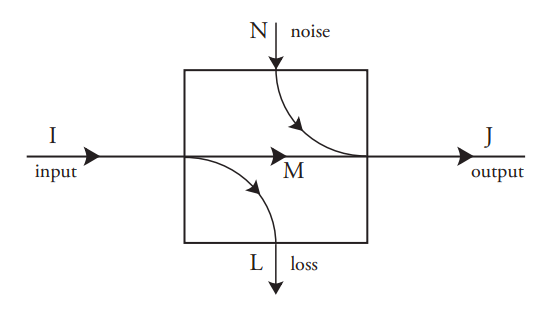
It is often necessary to determine the input event when only the output event has been observed. This is the case for communication systems, in which the objective is to infer the symbol emitted by the source so that it can be reproduced at the output. It is also the case for memory systems, in which the objective is to recreate the original bit pattern without error.

In principle, this estimation is straightforward if the input probability distribution \(p(A_i)\) and the conditional output probabilities, conditioned on the input events, \(p(B_j \;|\; A_i) = c_{ji}\), are known. These “forward” conditional probabilities \(c_{ji}\) form a matrix with as many rows as there are output events, and as many columns as there are input events. They are a property of the process, and do not depend on the input probabilities \(p(A_i)\).

The unconditional probability \(p(B_j)\) of each output event \(B_j\) is

\(p(B_j) = \displaystyle \sum_{i} c_{ji}p(A_i)\tag{8.1}\)

Figure 8.1: Information flow in a discrete memoryless process

and the joint probability of each input with each output \(p(A_i, B_j)\) and the backward conditional probabilities \(p(A_i \;|\; B_j)\) can be found using Bayes’ Theorem:

\begin{align*}
p(A_{i}, B_{j}) &=p(B_{j}) p(A_{i} \;|\; B_{j}) \\
&= p(A_{i}) p(B_{j} \;|\; A_{i}) \tag{8.2} \\
&=p(A_{i}) c_{ji}
\end{align*}

Now let us suppose that a particular output event \(B_j\) has been observed. The input event that “caused” this output can be estimated only to the extent of giving a probability distribution over the input events. For each input event \(A_i\) the probability that it was the input is simply the backward conditional probability \(p(A_i \;|\; B_j)\) for the particular output event \(B_j\), which can be written using Equation 8.2 as

\(p(A_i \;|\; B_j) = \dfrac{p(A_i)c_{ji}}{p(B_j)} \tag{8.3}\)

If the process has no loss (\(L\) = 0) then for each \(j\) exactly one of the input events \(A_i\) has nonzero probability, and therefore its probability \(p(A_i \;|\; B_j)\) is 1. In the more general case, with nonzero loss, estimation consists of refining a set of input probabilities so they are consistent with the known output. Note that this approach only works if the original input probability distribution is known. All it does is refine that distribution in the light of new knowledge, namely the observed output.

It might be thought that the new input probability distribution would have less uncertainty than that of the original distribution. Is this always true?

The uncertainty of a probability distribution is, of course, its entropy as defined earlier. The uncertainty (about the input event) before the output event is known is

\(U_{\text{before}} = \displaystyle \sum_{i} p(A_i) \log_2 \Big(\dfrac{1}{p(A_i)}\Big) \tag{8.4}\)

The residual uncertainty, after some particular output event is known, is

\(U_{\text{after}}(B_j) = \displaystyle \sum_{i} p(A_i \;|\; B_j) \log_2 \Big(\dfrac{1}{p(A_i \;|\; B_j)}\Big) \tag{8.5}\)

The question, then is whether \(U_{\text{after}}(B_j) ≤ U_{\text{before}}\). The answer is often, but not always, yes. However, it is not difficult to prove that the average (over all output states) of the residual uncertainty is less than the original uncertainty:

\(\displaystyle \sum_{j} p(B_j)U_{\text{after}}(B_j) ≤ U_{\text{before}} \tag{8.6}\)

(a)

(b)

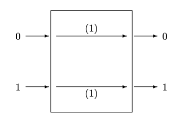
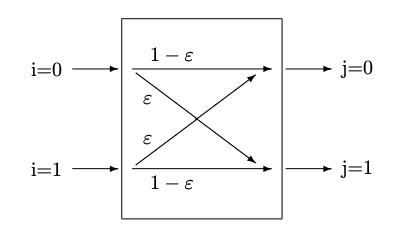
Figure 8.2: : (a) Binary Channel without noise (b) Symmetric Binary Channel, with errors

In words, this statement says that on average, our uncertainty about the input state is never increased by learning something about the output state. In other words, on average, this technique of inference helps us get a better estimate of the input state.

Two of the following examples will be continued in subsequent chapters including the next chapter on the Principle of Maximum Entropy—the symmetric binary channel and Berger’s Burgers.