9.1.2: Magnetic Dipole Model

An array of magnetic dipoles (think of them as tiny magnets) are subjected to an externally applied magnetic field \(H\) and therefore the energy of the system depends on their orientations and on the applied field. For simplicity our system contains only one such dipole, which from time to time is able to interchange information and energy with either of two environments, which are much larger collections of dipoles. Each

Table 9.1: Berger’s Burgers

Item	Entree	Cost	Calories	Probability of arriving hot	Probability of arriving cold
Meal 1	Burger	$1.00	1000	0.5	0.5
Meal 2	Chicken	$2.00	600	0.8	0.2
Meal 3	Fish	$3.00	400	0.9	0.1
Meal 4	Tofu	$4.00	200	0.6	0.4

Figure 9.1: Dipole moment example. (Each dipole can be either up or down.)

dipole, both in the system and in its two environments, can be either “up” or “down.” The system has one dipole so it only has two states, corresponding to the two states for that dipole, “up” and “down” (if the system had n dipoles it would have 2\(^n\) states). The energy of each dipole is proportional to the applied field and depends on its orientation; the energy of the system is the sum of the energies of all the dipoles in the system, in our case only one such.

Table 9.2: Magnetic Dipole Moments

State	Alignment	Energy
U	up	\(-m_dH\)
D	down	\(m_dH\)

The constant \(m_d\) is expressed in Joules per Tesla, and its value depends on the physics of the particular dipole. For example, the dipoles might be electron spins, in which case \(m_d = 2µ_Bµ_0\) where \(µ_0 = 4\pi × 10^{−7}\) henries per meter (in rationalized MKS units) is the permeability of free space, \(µ_B = \hbar e/2m_e = 9.272×10^{−24}\) Joules per Tesla is the Bohr magneton, and where \(\hbar = h/2\pi, h = 6.626 × 10^{−34}\) Joule-seconds is Plank’s constant, \(e = 1.602 × 10^{−19}\) coulombs is the magnitude of the charge of an electron, and \(m_e = 9.109 × 10^{−31}\) kilograms is the rest mass of an electron.

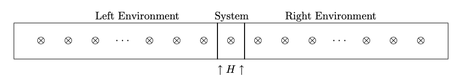
In Figure 9.1, the system is shown between two environments, and there are barriers between the environments and the system (represented by vertical lines) which prevent interaction (later we will remove the barriers to permit interaction). The dipoles, in both the system and the environments, are represented by the symbol \(\otimes\) and may be either spin-up or spin-down. The magnetic field shown is applied to the system only, not to the environments.

The virtue of a model with only one dipole is that it is simple enough that the calculations can be carried out easily. Such a model is, of course, hopelessly simplistic and cannot be expected to lead to numerically accurate results. A more realistic model would require so many dipoles and so many states that practical computations on the collection could never be done. For example, a mole of a chemical element is a small amount by everyday standards, but it contains Avogadro’s number \(N_A = 6.02252 × 10^{23}\) of atoms, and a correspondingly large number of electron spins; the number of possible states would be 2 raised to that power. Just how large this number is can be appreciated by noting that the earth contains no more than 2\(^{170}\) atoms, and the visible universe has about 2\(^{265}\) atoms; both of these numbers are way less than the number of states in that model. Even if we are less ambitious and want to compute with a much smaller sample, say 200 spins, and want to represent in our computer the probability of each state (using only 8 bits per state), we would still need more bytes of memory than there are atoms in the earth. Clearly it is impossible to compute with so many states, so the techniques described in these notes cannot be carried through in detail. Nevertheless there are certain conclusions and general relationships we will be able to establish.