Engineering LibreTexts

1.6: The Mass-Damper System III - Numerical and Graphical Evaluation of Time Response using MATLAB

  • Page ID
    21143
  • \( \newcommand{\vecs}[1]{\overset { \scriptstyle \rightharpoonup} {\mathbf{#1}} } \)

    \( \newcommand{\vecd}[1]{\overset{-\!-\!\rightharpoonup}{\vphantom{a}\smash {#1}}} \)

    \( \newcommand{\id}{\mathrm{id}}\) \( \newcommand{\Span}{\mathrm{span}}\)

    ( \newcommand{\kernel}{\mathrm{null}\,}\) \( \newcommand{\range}{\mathrm{range}\,}\)

    \( \newcommand{\RealPart}{\mathrm{Re}}\) \( \newcommand{\ImaginaryPart}{\mathrm{Im}}\)

    \( \newcommand{\Argument}{\mathrm{Arg}}\) \( \newcommand{\norm}[1]{\| #1 \|}\)

    \( \newcommand{\inner}[2]{\langle #1, #2 \rangle}\)

    \( \newcommand{\Span}{\mathrm{span}}\)

    \( \newcommand{\id}{\mathrm{id}}\)

    \( \newcommand{\Span}{\mathrm{span}}\)

    \( \newcommand{\kernel}{\mathrm{null}\,}\)

    \( \newcommand{\range}{\mathrm{range}\,}\)

    \( \newcommand{\RealPart}{\mathrm{Re}}\)

    \( \newcommand{\ImaginaryPart}{\mathrm{Im}}\)

    \( \newcommand{\Argument}{\mathrm{Arg}}\)

    \( \newcommand{\norm}[1]{\| #1 \|}\)

    \( \newcommand{\inner}[2]{\langle #1, #2 \rangle}\)

    \( \newcommand{\Span}{\mathrm{span}}\) \( \newcommand{\AA}{\unicode[.8,0]{x212B}}\)

    \( \newcommand{\vectorA}[1]{\vec{#1}}      % arrow\)

    \( \newcommand{\vectorAt}[1]{\vec{\text{#1}}}      % arrow\)

    \( \newcommand{\vectorB}[1]{\overset { \scriptstyle \rightharpoonup} {\mathbf{#1}} } \)

    \( \newcommand{\vectorC}[1]{\textbf{#1}} \)

    \( \newcommand{\vectorD}[1]{\overrightarrow{#1}} \)

    \( \newcommand{\vectorDt}[1]{\overrightarrow{\text{#1}}} \)

    \( \newcommand{\vectE}[1]{\overset{-\!-\!\rightharpoonup}{\vphantom{a}\smash{\mathbf {#1}}}} \)

    \( \newcommand{\vecs}[1]{\overset { \scriptstyle \rightharpoonup} {\mathbf{#1}} } \)

    \( \newcommand{\vecd}[1]{\overset{-\!-\!\rightharpoonup}{\vphantom{a}\smash {#1}}} \)

    \(\newcommand{\avec}{\mathbf a}\) \(\newcommand{\bvec}{\mathbf b}\) \(\newcommand{\cvec}{\mathbf c}\) \(\newcommand{\dvec}{\mathbf d}\) \(\newcommand{\dtil}{\widetilde{\mathbf d}}\) \(\newcommand{\evec}{\mathbf e}\) \(\newcommand{\fvec}{\mathbf f}\) \(\newcommand{\nvec}{\mathbf n}\) \(\newcommand{\pvec}{\mathbf p}\) \(\newcommand{\qvec}{\mathbf q}\) \(\newcommand{\svec}{\mathbf s}\) \(\newcommand{\tvec}{\mathbf t}\) \(\newcommand{\uvec}{\mathbf u}\) \(\newcommand{\vvec}{\mathbf v}\) \(\newcommand{\wvec}{\mathbf w}\) \(\newcommand{\xvec}{\mathbf x}\) \(\newcommand{\yvec}{\mathbf y}\) \(\newcommand{\zvec}{\mathbf z}\) \(\newcommand{\rvec}{\mathbf r}\) \(\newcommand{\mvec}{\mathbf m}\) \(\newcommand{\zerovec}{\mathbf 0}\) \(\newcommand{\onevec}{\mathbf 1}\) \(\newcommand{\real}{\mathbb R}\) \(\newcommand{\twovec}[2]{\left[\begin{array}{r}#1 \\ #2 \end{array}\right]}\) \(\newcommand{\ctwovec}[2]{\left[\begin{array}{c}#1 \\ #2 \end{array}\right]}\) \(\newcommand{\threevec}[3]{\left[\begin{array}{r}#1 \\ #2 \\ #3 \end{array}\right]}\) \(\newcommand{\cthreevec}[3]{\left[\begin{array}{c}#1 \\ #2 \\ #3 \end{array}\right]}\) \(\newcommand{\fourvec}[4]{\left[\begin{array}{r}#1 \\ #2 \\ #3 \\ #4 \end{array}\right]}\) \(\newcommand{\cfourvec}[4]{\left[\begin{array}{c}#1 \\ #2 \\ #3 \\ #4 \end{array}\right]}\) \(\newcommand{\fivevec}[5]{\left[\begin{array}{r}#1 \\ #2 \\ #3 \\ #4 \\ #5 \\ \end{array}\right]}\) \(\newcommand{\cfivevec}[5]{\left[\begin{array}{c}#1 \\ #2 \\ #3 \\ #4 \\ #5 \\ \end{array}\right]}\) \(\newcommand{\mattwo}[4]{\left[\begin{array}{rr}#1 \amp #2 \\ #3 \amp #4 \\ \end{array}\right]}\) \(\newcommand{\laspan}[1]{\text{Span}\{#1\}}\) \(\newcommand{\bcal}{\cal B}\) \(\newcommand{\ccal}{\cal C}\) \(\newcommand{\scal}{\cal S}\) \(\newcommand{\wcal}{\cal W}\) \(\newcommand{\ecal}{\cal E}\) \(\newcommand{\coords}[2]{\left\{#1\right\}_{#2}}\) \(\newcommand{\gray}[1]{\color{gray}{#1}}\) \(\newcommand{\lgray}[1]{\color{lightgray}{#1}}\) \(\newcommand{\rank}{\operatorname{rank}}\) \(\newcommand{\row}{\text{Row}}\) \(\newcommand{\col}{\text{Col}}\) \(\renewcommand{\row}{\text{Row}}\) \(\newcommand{\nul}{\text{Nul}}\) \(\newcommand{\var}{\text{Var}}\) \(\newcommand{\corr}{\text{corr}}\) \(\newcommand{\len}[1]{\left|#1\right|}\) \(\newcommand{\bbar}{\overline{\bvec}}\) \(\newcommand{\bhat}{\widehat{\bvec}}\) \(\newcommand{\bperp}{\bvec^\perp}\) \(\newcommand{\xhat}{\widehat{\xvec}}\) \(\newcommand{\vhat}{\widehat{\vvec}}\) \(\newcommand{\uhat}{\widehat{\uvec}}\) \(\newcommand{\what}{\widehat{\wvec}}\) \(\newcommand{\Sighat}{\widehat{\Sigma}}\) \(\newcommand{\lt}{<}\) \(\newcommand{\gt}{>}\) \(\newcommand{\amp}{&}\) \(\definecolor{fillinmathshade}{gray}{0.9}\)

    For the mass-damper response solution developed in the previous section, consider the following numerical case, with all quantities expressed in SI units: \(m\) = 5 kg, \(c\) = 2 N-s/m, \(F\) = 18 N, \(t_d\) = 7.5 s, \(v_0\) = 3.3 m/s. A MATLAB script M-file, named MATLABdemo11.m, to calculate and graph the response from 0 to 25 seconds is given below. The MATLAB commands are supplemented with explanatory comments, so you should be able to follow and understand the M-file without much difficulty. Writing comments in this manner is good practice for your own programs; comments added while you are writing a computer program are especially helpful if you need to revise or refer back to the program long after you have forgotten the details.

    %MATLABdemo11.m
    
    %Mass-damper system response to IC + half-sine pulse forcing
    
    m=5;c=2; %system mass & viscous damping coefficient, SI units
    
    F=18;td=7.5; %half-sine pulse, amplitude (N), pulse duration (sec)
    
    vo=3.3; %initial velocity (m/sec)
    
    w=pi/td; %circular frequency of half-sine pulse (rad/sec)
    
    t1=0:0.05:td; %time instants for forced response
    
    f1=F*sin(w*t1); %force pulse
    
    P1=c*F/((w*m)^2+c^2); P2=P1*(-w*m/c);C=vo-P2; %constants
    
    v1=C*exp(-c/m*t1)+P1*sin(w*t1)+P2*cos(w*t1);%time series of forced velocity
    
    nt1end=length(t1);v2o=v1(nt1end);%initial velocity for post-pulse response
    
    t2=td:0.1:25; %time instants for post-pulse unforced response
    
    v2=v2o*exp(-c/m*(t2-td));%time series of post-pulse unforced velocity
    
    f2=zeros(1,length(t2)); %null force after pulse
    
    plot(t1,f1/10,'k',t1,v1,'k',t2,f2,'k',t2,v2,'k'),grid,xlabel('Time t (sec)')
    
    ylabel('Force f_x(t) (daN), and Velocity v(t) (m/sec)')
    
    title('Response of mass-damper system to IC + half-sine pulse forcing')

    To execute in MATLAB an M-file that is stored on a folder (directory) of your computer’s hard disk, you must have added that folder to the so-called MATLABpath. In Versions 6 and higher of MATLAB, you can add the folder to the MATLABpath by specifying the folder as the “Current Directory” in the formatting toolbar above the MATLAB command window. The command line below executes the script M-file.

    MATLAB command:

    >> MATLABdemo11

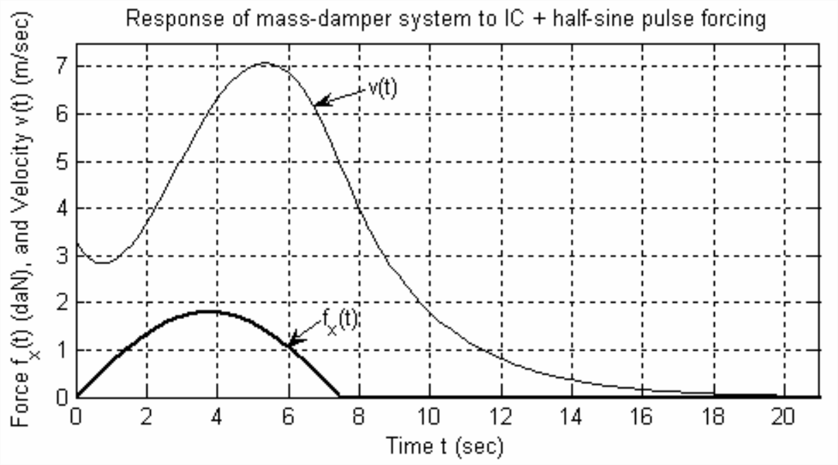
    The resulting MATLAB (Versions 6 and higher) graph is Figure \(\PageIndex{1}\). The graph was edited in the MATLAB figure window, mainly to reduce the size and to add curve labels and arrows.

    Note that the unit of force “daN” on Figure \(\PageIndex{1}\) is a deka-newton, which means 10 newtons. All of the mechanical units used in this book are described in Chapter 3.
    clipboard_eb9aab701074c321cfda8c9d186757a3c.png
    Figure \(\PageIndex{1}\): Excitation and response of a mass-damper system

    This page titled 1.6: The Mass-Damper System III - Numerical and Graphical Evaluation of Time Response using MATLAB is shared under a CC BY-NC 4.0 license and was authored, remixed, and/or curated by William L. Hallauer Jr. (Virginia Tech Libraries' Open Education Initiative) via source content that was edited to the style and standards of the LibreTexts platform.