Engineering LibreTexts

8.7: Ideal Impulse Response of an Undamped Second Order System

  • Page ID
    8039
  • \( \newcommand{\vecs}[1]{\overset { \scriptstyle \rightharpoonup} {\mathbf{#1}} } \)

    \( \newcommand{\vecd}[1]{\overset{-\!-\!\rightharpoonup}{\vphantom{a}\smash {#1}}} \)

    \( \newcommand{\id}{\mathrm{id}}\) \( \newcommand{\Span}{\mathrm{span}}\)

    ( \newcommand{\kernel}{\mathrm{null}\,}\) \( \newcommand{\range}{\mathrm{range}\,}\)

    \( \newcommand{\RealPart}{\mathrm{Re}}\) \( \newcommand{\ImaginaryPart}{\mathrm{Im}}\)

    \( \newcommand{\Argument}{\mathrm{Arg}}\) \( \newcommand{\norm}[1]{\| #1 \|}\)

    \( \newcommand{\inner}[2]{\langle #1, #2 \rangle}\)

    \( \newcommand{\Span}{\mathrm{span}}\)

    \( \newcommand{\id}{\mathrm{id}}\)

    \( \newcommand{\Span}{\mathrm{span}}\)

    \( \newcommand{\kernel}{\mathrm{null}\,}\)

    \( \newcommand{\range}{\mathrm{range}\,}\)

    \( \newcommand{\RealPart}{\mathrm{Re}}\)

    \( \newcommand{\ImaginaryPart}{\mathrm{Im}}\)

    \( \newcommand{\Argument}{\mathrm{Arg}}\)

    \( \newcommand{\norm}[1]{\| #1 \|}\)

    \( \newcommand{\inner}[2]{\langle #1, #2 \rangle}\)

    \( \newcommand{\Span}{\mathrm{span}}\) \( \newcommand{\AA}{\unicode[.8,0]{x212B}}\)

    \( \newcommand{\vectorA}[1]{\vec{#1}}      % arrow\)

    \( \newcommand{\vectorAt}[1]{\vec{\text{#1}}}      % arrow\)

    \( \newcommand{\vectorB}[1]{\overset { \scriptstyle \rightharpoonup} {\mathbf{#1}} } \)

    \( \newcommand{\vectorC}[1]{\textbf{#1}} \)

    \( \newcommand{\vectorD}[1]{\overrightarrow{#1}} \)

    \( \newcommand{\vectorDt}[1]{\overrightarrow{\text{#1}}} \)

    \( \newcommand{\vectE}[1]{\overset{-\!-\!\rightharpoonup}{\vphantom{a}\smash{\mathbf {#1}}}} \)

    \( \newcommand{\vecs}[1]{\overset { \scriptstyle \rightharpoonup} {\mathbf{#1}} } \)

    \( \newcommand{\vecd}[1]{\overset{-\!-\!\rightharpoonup}{\vphantom{a}\smash {#1}}} \)

    \(\newcommand{\avec}{\mathbf a}\) \(\newcommand{\bvec}{\mathbf b}\) \(\newcommand{\cvec}{\mathbf c}\) \(\newcommand{\dvec}{\mathbf d}\) \(\newcommand{\dtil}{\widetilde{\mathbf d}}\) \(\newcommand{\evec}{\mathbf e}\) \(\newcommand{\fvec}{\mathbf f}\) \(\newcommand{\nvec}{\mathbf n}\) \(\newcommand{\pvec}{\mathbf p}\) \(\newcommand{\qvec}{\mathbf q}\) \(\newcommand{\svec}{\mathbf s}\) \(\newcommand{\tvec}{\mathbf t}\) \(\newcommand{\uvec}{\mathbf u}\) \(\newcommand{\vvec}{\mathbf v}\) \(\newcommand{\wvec}{\mathbf w}\) \(\newcommand{\xvec}{\mathbf x}\) \(\newcommand{\yvec}{\mathbf y}\) \(\newcommand{\zvec}{\mathbf z}\) \(\newcommand{\rvec}{\mathbf r}\) \(\newcommand{\mvec}{\mathbf m}\) \(\newcommand{\zerovec}{\mathbf 0}\) \(\newcommand{\onevec}{\mathbf 1}\) \(\newcommand{\real}{\mathbb R}\) \(\newcommand{\twovec}[2]{\left[\begin{array}{r}#1 \\ #2 \end{array}\right]}\) \(\newcommand{\ctwovec}[2]{\left[\begin{array}{c}#1 \\ #2 \end{array}\right]}\) \(\newcommand{\threevec}[3]{\left[\begin{array}{r}#1 \\ #2 \\ #3 \end{array}\right]}\) \(\newcommand{\cthreevec}[3]{\left[\begin{array}{c}#1 \\ #2 \\ #3 \end{array}\right]}\) \(\newcommand{\fourvec}[4]{\left[\begin{array}{r}#1 \\ #2 \\ #3 \\ #4 \end{array}\right]}\) \(\newcommand{\cfourvec}[4]{\left[\begin{array}{c}#1 \\ #2 \\ #3 \\ #4 \end{array}\right]}\) \(\newcommand{\fivevec}[5]{\left[\begin{array}{r}#1 \\ #2 \\ #3 \\ #4 \\ #5 \\ \end{array}\right]}\) \(\newcommand{\cfivevec}[5]{\left[\begin{array}{c}#1 \\ #2 \\ #3 \\ #4 \\ #5 \\ \end{array}\right]}\) \(\newcommand{\mattwo}[4]{\left[\begin{array}{rr}#1 \amp #2 \\ #3 \amp #4 \\ \end{array}\right]}\) \(\newcommand{\laspan}[1]{\text{Span}\{#1\}}\) \(\newcommand{\bcal}{\cal B}\) \(\newcommand{\ccal}{\cal C}\) \(\newcommand{\scal}{\cal S}\) \(\newcommand{\wcal}{\cal W}\) \(\newcommand{\ecal}{\cal E}\) \(\newcommand{\coords}[2]{\left\{#1\right\}_{#2}}\) \(\newcommand{\gray}[1]{\color{gray}{#1}}\) \(\newcommand{\lgray}[1]{\color{lightgray}{#1}}\) \(\newcommand{\rank}{\operatorname{rank}}\) \(\newcommand{\row}{\text{Row}}\) \(\newcommand{\col}{\text{Col}}\) \(\renewcommand{\row}{\text{Row}}\) \(\newcommand{\nul}{\text{Nul}}\) \(\newcommand{\var}{\text{Var}}\) \(\newcommand{\corr}{\text{corr}}\) \(\newcommand{\len}[1]{\left|#1\right|}\) \(\newcommand{\bbar}{\overline{\bvec}}\) \(\newcommand{\bhat}{\widehat{\bvec}}\) \(\newcommand{\bperp}{\bvec^\perp}\) \(\newcommand{\xhat}{\widehat{\xvec}}\) \(\newcommand{\vhat}{\widehat{\vvec}}\) \(\newcommand{\uhat}{\widehat{\uvec}}\) \(\newcommand{\what}{\widehat{\wvec}}\) \(\newcommand{\Sighat}{\widehat{\Sigma}}\) \(\newcommand{\lt}{<}\) \(\newcommand{\gt}{>}\) \(\newcommand{\amp}{&}\) \(\definecolor{fillinmathshade}{gray}{0.9}\)

    The ODE for a standard undamped 2nd order system is \(\ddot{x}+\omega_{n}^{2} x=\omega_{n}^{2} u(t)\). Let the input function be the ideal impulse, \(u(t)=I_{U} \delta(t)\), and let the pre-impulse initial conditions be \(x\left(0^{-}\right) \equiv x_{0}\), \(\dot{x}\left(0^{-}\right) \equiv \dot{x}_{0}\). Just as for the 1st order system with ideal-impulse excitation in Section 8.5, we will solve the present problem by the conventional Laplace-transform approach. Note that we will use the second derivative form of Equation 8.6.4: \(L[\ddot{f}]=s^{2} F(s)-s f\left(0^{-}\right)-\dot{f}\left(0^{-}\right)\). With \(L[\delta(t)]=1\) from Equation 8.4.6, the steps of the solution are:

    \[L[\mathrm{ODE}]: \quad s^{2} X(s)-s x_{0}-\dot{x}_{0}+\omega_{n}^{2} X(s)=b U(s)=\omega_{n}^{2} I_{U} \times 1 \nonumber \]

    \[\Rightarrow \quad X(s)=\frac{\omega_{n}^{2} I_{U}+\dot{x}_{0}+s x_{0}}{s^{2}+\omega_{n}^{2}}=\left(\omega_{n} I_{U}+\frac{\dot{x}_{0}}{\omega_{n}}\right) \frac{\omega_{n}}{s^{2}+\omega_{n}^{2}}+x_{0} \frac{s}{s^{2}+\omega_{n}^{2}}\label{eqn:8.25} \]

    \[\Rightarrow \quad x(t)=\left(\omega_{n} I_{U}+\frac{\dot{x}_{0}}{\omega_{n}}\right) \sin \omega_{n} t+x_{0} \cos \omega_{n} t, t \geq 0^{+}\label{eqn:8.26} \]

    At the risk of being excessively repetitive, we emphasize that the discussions in Sections 8.5 and 8.6 show that response Equation \(\ref{eqn:8.26}\) is the post-impulse solution, certainly valid mathematically for \(t \geq 0^{+}\), but not necessarily correct, in particular, for the pre-impulse initial conditions at \(t=0^-\).

    Solution Equation \(\ref{eqn:8.26}\) holds for a general undamped 2nd order system; let us adapt it specifically to a mass-spring system, with zero initial conditions, that is hit by an ideal impulse of force having magnitude \(I_{F}\), with units, for example, of N-s or lb-s. From Equation 7.1.4, we find

    \[u(t)=f_{x}(t) / k \Rightarrow I_{U} \delta(t)=I_{F} \delta(t) / k \Rightarrow I_{U}=I_{F} / k\label{eqn:8.27} \]

    So, for translational motion \(x(t)\) of the mass, Equation \(\ref{eqn:8.26}\) with zero initial conditions becomes (recall \(k=m \omega_{n}^{2}\))

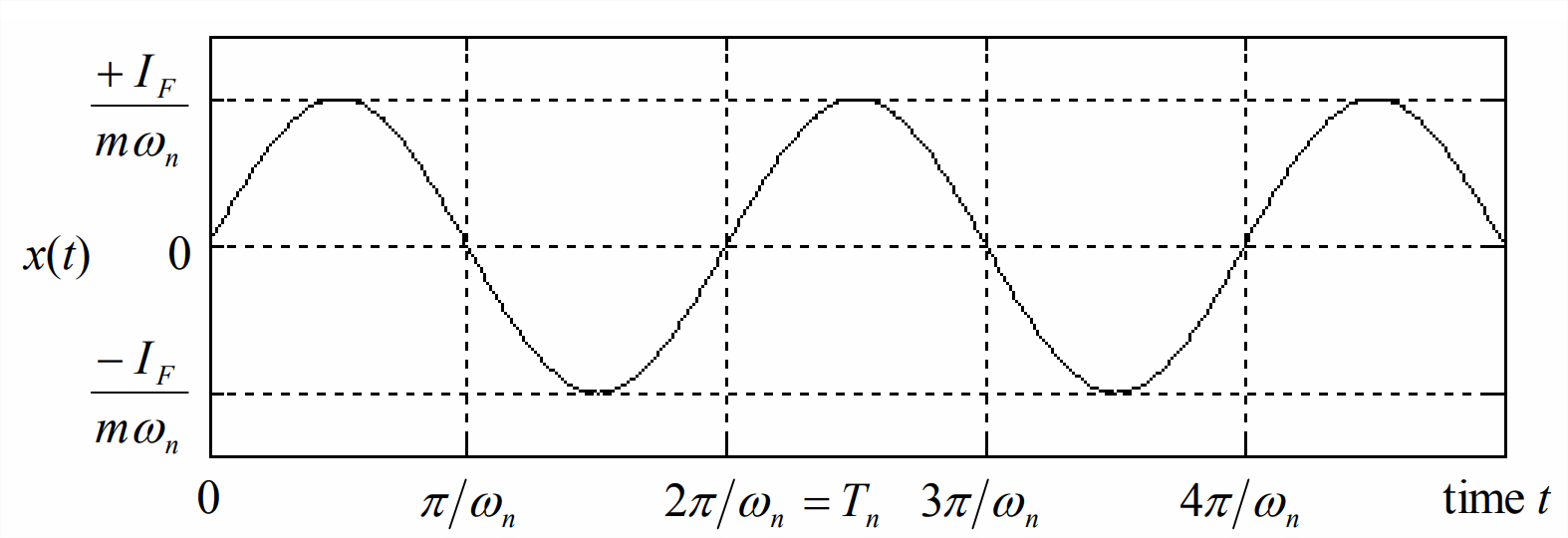
    \[x(t)=\omega_{n} \frac{I_{F}}{k} \sin \omega_{n} t=\frac{I_{F}}{m \omega_{n}} \sin \omega_{n} t\label{eqn:8.28} \]

    Figure \(\PageIndex{1}\) shows a few cycles of response Equation \(\ref{eqn:8.28}\).
    clipboard_ea6beee625d01d804e3421ce39269126d.png
    Figure \(\PageIndex{1}\): Ideal impulse response of a mass-spring system

    This page titled 8.7: Ideal Impulse Response of an Undamped Second Order System is shared under a CC BY-NC 4.0 license and was authored, remixed, and/or curated by William L. Hallauer Jr. (Virginia Tech Libraries' Open Education Initiative) via source content that was edited to the style and standards of the LibreTexts platform.