13.1: Laplace Block Diagrams for an RC Band-Pass Filter

Last updated
Save as PDF

Page ID: 7705

\( \newcommand{\vecs}[1]{\overset { \scriptstyle \rightharpoonup} {\mathbf{#1}} } \) \( \newcommand{\vecd}[1]{\overset{-\!-\!\rightharpoonup}{\vphantom{a}\smash {#1}}} \)\(\newcommand{\id}{\mathrm{id}}\) \( \newcommand{\Span}{\mathrm{span}}\) \( \newcommand{\kernel}{\mathrm{null}\,}\) \( \newcommand{\range}{\mathrm{range}\,}\) \( \newcommand{\RealPart}{\mathrm{Re}}\) \( \newcommand{\ImaginaryPart}{\mathrm{Im}}\) \( \newcommand{\Argument}{\mathrm{Arg}}\) \( \newcommand{\norm}[1]{\| #1 \|}\) \( \newcommand{\inner}[2]{\langle #1, #2 \rangle}\) \( \newcommand{\Span}{\mathrm{span}}\) \(\newcommand{\id}{\mathrm{id}}\) \( \newcommand{\Span}{\mathrm{span}}\) \( \newcommand{\kernel}{\mathrm{null}\,}\) \( \newcommand{\range}{\mathrm{range}\,}\) \( \newcommand{\RealPart}{\mathrm{Re}}\) \( \newcommand{\ImaginaryPart}{\mathrm{Im}}\) \( \newcommand{\Argument}{\mathrm{Arg}}\) \( \newcommand{\norm}[1]{\| #1 \|}\) \( \newcommand{\inner}[2]{\langle #1, #2 \rangle}\) \( \newcommand{\Span}{\mathrm{span}}\)\(\newcommand{\AA}{\unicode[.8,0]{x212B}}\)

To introduce the Laplace block diagram for a simple case, we re-visit again the \(RC\) band-pass filter considered previously in Sections 5.4, 9.10, and 10.4. As shown in Fig. 5.4.1, this circuit consists of a low-pass-filter stage to the left of the voltage follower, and a high-pass-filter stage to the right. The Laplace transforms derived for these stages in Section 10.4, assuming zero ICs, are: for the low-pass stage, with \(\tau_{L}=R_{L} C_{L}\),

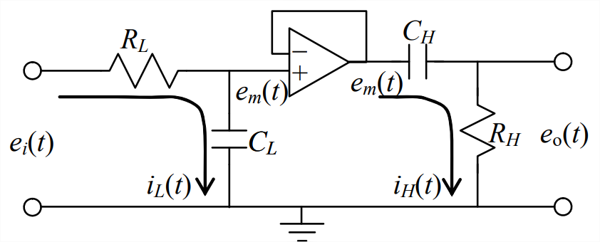
Figure \(\PageIndex{1}\): (repeated) \(RC\) band-pass filter. (Copyright; author via source)

\[L\left[e_{m}\right]=\frac{1}{\tau_{L} s+1} L\left[e_{i}\right]\label{eqn:13.1} \]

and for the high-pass stage, with \(\tau_{H}=R_{H} C_{H}\),

\[L\left[e_{o}\right]=\frac{\tau_{H} S}{\tau_{H} s+1} L\left[e_{m}\right]\label{eqn:13.2} \]

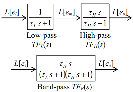
Figure \(\PageIndex{2}\): Laplace block diagrams of the \(RC\) band-pass filter. (Copyright; author via source)

Figure \(\PageIndex{2}\) shows a convenient graphical format, the block diagram, for representing these Laplace-transform output-to-input relationships. From Equations \(\ref{eqn:13.1}\) and \(\ref{eqn:13.2}\), we have the individual transfer functions of the low-pass and high-pass stages:

\[T F_{L}(s)=\frac{L\left[e_{m}\right]}{L\left[e_{i}\right]}=\frac{1}{\tau_{L} s+1}\label{eqn:13.3} \]

\[T F_{H}(s)=\frac{L\left[e_{o}\right]}{L\left[e_{m}\right]}=\frac{\tau_{H} s}{\tau_{H} s+1}\label{eqn:13.4} \]

In the upper row of Figure \(\PageIndex{2}\), transfer functions Equations \(\ref{eqn:13.3}\) and \(\ref{eqn:13.4}\) are shown as individual blocks, and the Laplace transforms are shown as input and output “signals” relative to the blocks. The most basic rule of “block-diagram algebra” is that the input signal (transform) multiplied by the block transfer function equals the output signal (transform), which gives Equations \(\ref{eqn:13.1}\) and \(\ref{eqn:13.2}\).

One common objective in construction of Laplace block diagrams is to simplify the process of deriving the transfer function of the overall system from the transfer functions of individual sub-systems. To help achieve this objective, we have the second basic rule of block-diagram algebra: multiply the transfer functions of two adjacent blocks in order to obtain the more general transfer function relating the output signal from the downstream block to the input signal into the upstream block. The result of this operation in the present case is shown in the lower row of Figure \(\PageIndex{2}\), where transfer function Equation 10.4.4 of the entire \(RC\) band-pass filter circuit is derived once again:

\[T F_{B}(s)=\frac{L\left[e_{o}\right]}{L\left[e_{i}\right]}=\frac{\tau_{H} s}{\left(\tau_{H} s+1\right)\left(\tau_{L} s+1\right)}\label{eqn:13.5} \]

Each of the block diagrams in Figure \(\PageIndex{2}\) has a single forward (left-to-right) path or branch. A more general type of block diagram has a forward branch and also one or more backward paths denoting signal flow in the opposite direction; such a right-to-left path is called a feedback branch. A forward branch combined with a feedback branch forms a closed loop, and a block diagram that includes closed loops is called a closed-loop block diagram. Accordingly, a block diagram with only a forward branch is called an open-loop block diagram. The next section develops the concept of closed-loop block diagrams in the context of a familiar mechanical system.