13.2: Laplace Block Diagram with Feedback Branches

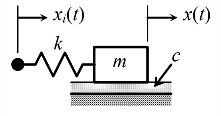
Let us proceed beyond the most basic aspects of Laplace block diagrams by analyzing the \(m\)-\(c\)-\(k\) system with base excitation shown on Figure \(\PageIndex{1}\). The input is base translation \(x_i(t)\), and the output is mass translation \(x(t)\). The ODE of motion for this system (from homework Problem 9.1) is

\[m \ddot{x}+c \dot{x}+k x=k x_{i}(t)\label{eqn:13.6} \]

Figure \(\PageIndex{1}\): \(m\)-\(c\)-\(k\) system with base excitation. (Copyright; author via source)

It is convenient to denote the input transform as \(L\left[x_{i}(t)\right]=X_{i}(s)\) and the output transform as \(L[x(t)]=X(s)\). Taking the Laplace transform of Equation \(\ref{eqn:13.6}\) with zero ICs, for the purpose of deriving the transfer function, gives

\[m s^{2} X(s)+c s X(s)+k X(s)=k X_{i}(s)\label{eqn:13.7} \]

Equation \(\ref{eqn:13.7}\) clearly leads to the transfer function,

\[T F(s) \equiv \frac{X(s)}{X_{i}(s)}=\frac{k}{m s^{2}+c s+k}\label{eqn:13.8} \]

Figure \(\PageIndex{2}\) (Copyright; author via source)

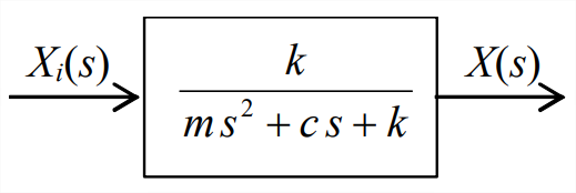
Equation \(\ref{eqn:13.8}\) is represented in the simple open-loop Laplace block diagram just above.

It will be instructive for our later study of feedback control to develop now an alternative but equivalent block diagram from Equation \(\ref{eqn:13.7}\). First, we transpose to the righthand side all terms other than the \(X(s)\) term of highest order:

\[m s^{2} X(s)=k X_{i}(s)-c s X(s)-k X(s)\label{eqn:13.9} \]

Now we “solve” algebraically for \(X(s)\) on the left-hand side of Equation \(\ref{eqn:13.9}\) simply by dividing through by the coefficient of the left-hand-side \(X(s)\):

\[X(s)=\frac{1}{s}\left\{\frac{1}{m s}\left[k X_{i}(s)-k X(s)-c s X(s)\right]\right\}\label{eqn:13.10} \]

Observe in Equation \(\ref{eqn:13.10}\) that output transform \(X(s)\) appears in the right-hand-side terms as well as on the left-hand side; these right-hand-side terms imply feedback. Using Equation \(\ref{eqn:13.10}\) leads to the following block diagram with several different transfer-function blocks and with two feedback branches:

Figure \(\PageIndex{3}\): Laplace block diagram with feedback branches for a base-excited \(m\)-\(c\)-\(k\) system (Copyright; author via source)

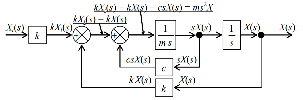
The input and output signals for every block are labeled on Figure \(\PageIndex{3}\) in order to help you relate the block diagram to Equation \(\ref{eqn:13.10}\), and you should carefully compare the equation and the diagram until you are certain that you understand.

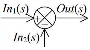
Also, block diagram Figure \(\PageIndex{3}\) introduces two kinds of junctions. The first kind is a simple branch point (black circle), from which the same blockoutput “signal” travels onward on two different branches, as is indicated by the signal labels on Figure \(\PageIndex{3}\). The second kind is a summing junction, shown at right with input and output signals labeled. This summing junction is configured for negative feedback, so it differences the two input signals, \(\operatorname{Out}(s)=\operatorname{In}_{1}(s)-\operatorname{In}_{2}(s)\).

Figure \(\PageIndex{4}\) (Copyright; author via source)

In this section, we started with ODE Equation \(\ref{eqn:13.6}\) and developed from it Laplace block diagram Figure \(\PageIndex{3}\). This approach is primarily for the purpose of presenting some important features of block diagrams. This approach is actually the reverse of the standard procedure for analysis of feedback-control systems, which we will consider in later chapters. There, we will start with the block diagram of a system, something like Figure \(\PageIndex{3}\), and derive from it the closed-loop transfer function, CLTF(s) ), which in this case is just Equation \(\ref{eqn:13.8}\). The process of deriving \(CLTF(s)\) from the system block diagram will require some new operations in block-diagram algebra; it is expedient to postpone the descriptions of these operations until we need them in later chapters.