13.3: Forced Response of an m-c-k System with Base Excitation

It will be helpful for our introduction to feedback control in Chapter 14 if we now examine the relationship between input motion \(x_{i}(t)\) and output motion \(x(t)\) for the mechanical system of Figure 13.2.1 and Equation 13.2.1. Let us adopt the perspective here that we want to use \(x_{i}(t)\) in order to control \(x(t)\); in particular for this system, let us suppose that we want to make motion \(x(t)\) of mass \(m\) be as close as possible to input motion \(x_{i}(t)\). You can visualize intuitively from Figure 13.2.1 that if \(x_{i}(t)\) is imposed very slowly, then \(x(t)\) will be essentially the same as \(x_{i}(t)\); in this case, the inertial force of mass \(m\) will be negligible, and spring \(k\) will deform only slightly, therefore acting essentially as a rigid link. (You can, of course, prove theoretically this qualitative analysis, for example, by finding frequency response at a very low input frequency.)

But can output motion \(x(t)\) be made close to input \(x_{i}(t)\) if \(x_{i}(t)\) is not imposed slowly? Your intuition probably fails to answer this question because, in this case, spring \(k\) might deform significantly, and the inertial force of mass \(m\) might not be negligible. We will have to analyze this situation theoretically. Let us do so specifying that input motion \(x_{i}(t)\) is a step function of magnitude \(X_{H}\) imposed at time \(t\) = 0. An ideal step input is not merely fast; it is in fact the fastest imaginable (though not physically realizable) base excitation, because base position changes with infinite velocity at \(t\) = 0 from \(x_{i}=0\) to \(x_{i}=X_{H}\). So this ideal input poses a formidable challenge to the control objective: can output translation \(x(t)\) approximate in some reasonable manner the input translation \(x_{i}(t)\), even though initially the input translation is infinitely fast?

In order to analyze this case, let us first adapt ODE Equation 13.2.1 to the standard ODE for damped 2^nd order systems as it is defined in Chapter 9. Dividing Equation 13.2.1 through by \(m\), and then applying the standard definitions Equation 7.1.3 for undamped natural frequency, \(\omega_{n}=\sqrt{k / m}\), and Equation 9.1.6 for viscous damping ratio, \(\zeta=c /(2 \sqrt{m k})\), casts the ODE into the form \(\ddot{x}+2 \zeta \omega_{n} \dot{x}+\omega_{n}^{2} x=\omega_{n}^{2} x_{i}(t)\). Comparing this ODE with Equation 9.2.2 shows that input \(x_{i}(t)\) for this particular base-excited \(m\)-\(c\)-\(k\) system is exactly equal to the standard input quantity: \(x_{i}(t) \equiv u(t)\). We define step input \(x_{i}(t)=X_{H} H(t)\). Therefore, \(X_{H} \equiv U\), which is the general step-input magnitude of Section 9.6, and we can write the step-response solution for \(|\zeta|<1\) directly from Equation 9.6.5:

\[x(t)=X_{H}\left[1-e^{-\zeta \omega_{n} t}\left(\cos \omega_{d} t+\frac{\zeta \omega_{n}}{\omega_{d}} \sin \omega_{d} t\right)\right], \text { for } 0 \leq t\label{eqn:13.11} \]

In Equation \(\ref{eqn:13.11}\), the damped natural frequency is \(\omega_{d} \equiv \omega_{n} \sqrt{1-\zeta^{2}}\). Also, for use in Figure \(\PageIndex{1}\), the period of the undamped system is \(T_{n}=2 \pi / \omega_{n}\). Recall that our control objective is to make the output motion at least approximately equal to the input motion. At \(t = 0\), input motion \(x_{i}(t)\) jumps discontinuously from 0 to \(X_{H}\), then \(x_i\) remains constant thereafter, so we would like the output motion \(x(t)\) to approximate that step input as closely as possible. In particular, we want the final, steady-state value of \(x(t)\) to be \(X_{H}\).

It is instructive to calculate and graph Equation \(\ref{eqn:13.11}\) for a few different values of \(\zeta\), assuming that the system is underdamped, \(0 \leq \zeta<1\). The step-response graphs are shown on Figure \(\PageIndex{1}\). If the system is undamped, \(c = 0\), then the mass oscillates forever (in theory) about the desired final position, \(x=X_{H}\); in this ideal (with zero damping) case, the control objective cannot be achieved.

Figure \(\PageIndex{1}\): Base-excitation control of mass position for an \(m\)-\(c\)-\(k\) system. (Copyright; author via source)

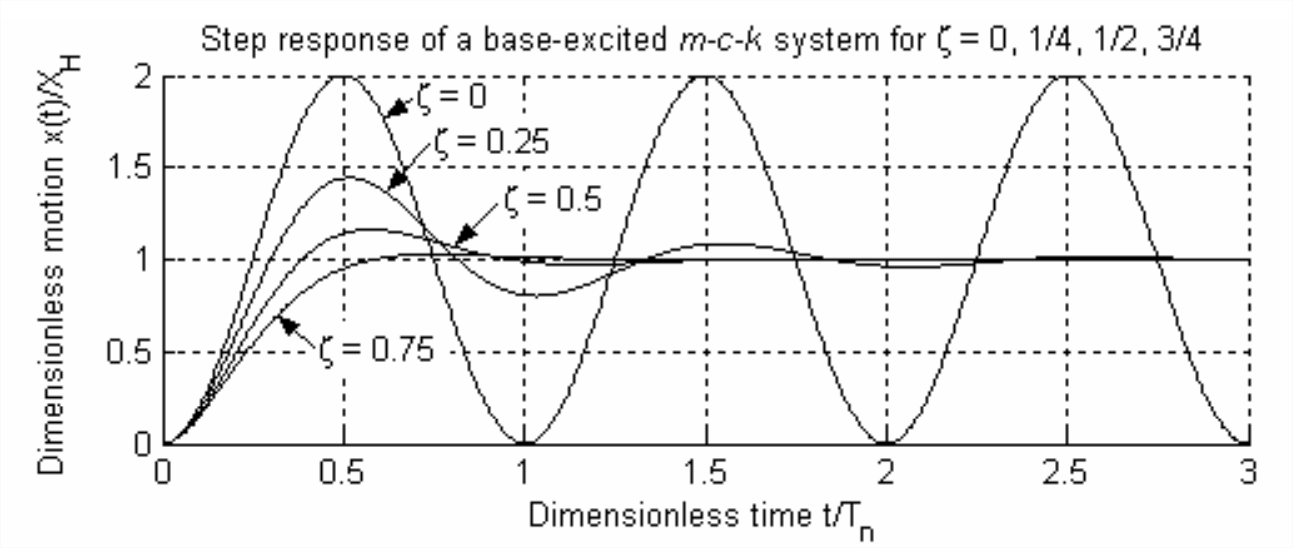
However, Figure \(\PageIndex{1}\) also demonstrates that, if there is positive damping, \(\zeta>0\), then the motion output \(x(t)\) does, indeed, approximate the step input, \(x_{i}(t)=X_{H} H(t)\): \(x(t)\) rises from 0, though with finite velocity, and it eventually settles at the desired final value, \(x=X_{H}\).

Note that the equations for step-response specifications (rise time, peak time, maximum overshoot ratio, and settling time) derived in Section 9.8 are applicable to this case of excitation of an \(m\)-\(c\)-\(k\) system by base motion.

The base-excited mass-damper-spring system of Figure 13.2.1 is an instructive prototype for output feedback control of mechanical position, which is the subject of Chapter 14. Therefore, we shall refer back to this system and to the results of Sections 13.2 and 13.3 in order to clarify and justify some of the control-system developments presented in Chapter 14.