17.1: Gain Margins, Phase Margins, and Bode Diagrams

In order to describe and illustrate the most basic form of frequency-response stability analysis, we consider again a familiar system from Chapter 16: the rotor position-feedback control system with a 1^st order low-pass filter in the feedback branch, for which the functional diagram is Figure 16.3.1 and the block diagram is Figure 16.3.2. We have already studied this system to determine absolute stability by Routh’s criteria in Section 16.3, and relative stability by calculating loci of roots and by applying the root-locus method in Sections 16.5 and 16.6. Knowing the stability characteristics in advance will guide us in interpreting the frequency-response analysis.

Figure \(\PageIndex{1}\) (Copyright; author via source)

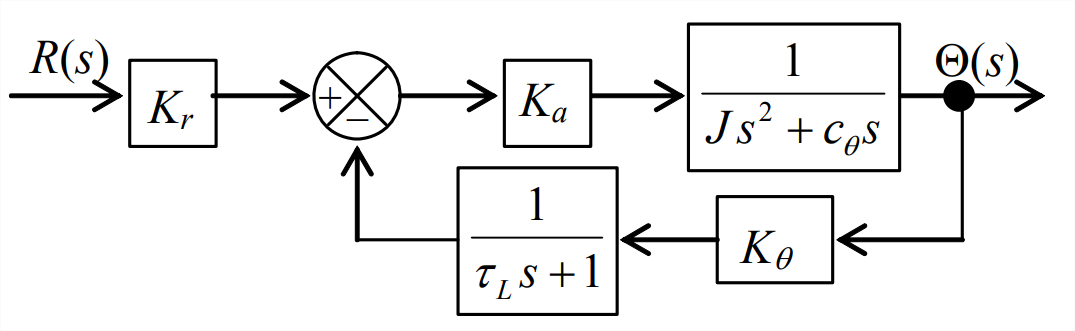
The branch transfer functions for the loop in Figure 16.3.2 are

\[G(s)=\frac{K_{a}}{J s^{2}+c_{\theta} s} \quad \text { and } \quad H(s)=\frac{K_{\theta}}{\tau_{L} s+1}\label{eqn:17.1} \]

The closed-loop transfer function is \(C L T F(s)=G(s) /[1+G(s) H(s)]\); the denominator of \(\operatorname{CLTF}(s)\) in this form for the system of Figure 16.3.2 is

\[1+G(s) H(s)=1+\frac{K_{a}}{J s^{2}+c_{\theta} s} \times \frac{K_{\theta}}{\tau_{L} s+1}=1+\frac{K_{a} K_{\theta}}{J} \frac{1 / \tau_{L}}{s\left(s+c_{\theta} / J\right)\left(s+1 / \tau_{L}\right)} \equiv 1+\Lambda \frac{\omega_{b}}{s\left(s+c_{\theta} / J\right)\left(s+\omega_{b}\right)} \equiv 1+O \operatorname{LTF}(s)\label{eqn:17.2} \]

where \(\Lambda \equiv K_{a} K_{\theta} / J\) is the control parameter, which we now call gain. We evaluate the stability of the closed-loop system as \(\Lambda\) ranges from 0 to \(+\inf\). The system constants from Chapter 16 are \(\omega_{b} \equiv 1 / \tau_{L}=300\) rad/s and \(c_{\theta} / J\) = 100 s^-1. In Section 16.5, we solved the characteristic equation of the closed-loop system, \(1+G(s) H(s)=0\).¹ We know from the loci of roots calculated for this system that, with gain \(\Lambda\) positive and increasing, there is a particular value of \(\Lambda\) for which the oscillatory loci of roots intersect the \(\operatorname{Im}[s]\) axis; for this value of \(\Lambda\), the oscillatory time response is purely sinusoidal and periodic, without any exponential envelope. Let us define that intersection as the point of oscillatory neutral stability and denote the value of \(\Lambda\) there as \(\Lambda_{n s}\) (the same as \(\Lambda_{u b}\) in Section 16.5). Accordingly, let us denote the oscillatory frequency at that point as \(\omega_{n s}\) (the same as \(\omega_{d}\) in Section 16.5). We determined in Chapter 16 that \(\Lambda_{n s}=\left(c_{\theta} / J\right) \times \left(c_{\theta} / J+\omega_{b}\right)=40,000\) s^-2 and \(\omega_{n s}=\sqrt{\left(c_{\theta} / J\right) \omega_{b}}=173.2\) rad/s, and that the closed-loop system is exponentially stable for \(0<\Lambda<\Lambda_{n s}\), but unstable for \(\Lambda>\Lambda_{n s}\).

The loci of roots are defined by the characteristic equation:

\[1+G(s) H(s) \equiv 1+O \operatorname{LTF}(s)=0\label{eqn:17.3} \]

Therefore, at the point of neutral stability, with \(\Lambda=\Lambda_{n s}\) and \(s=j \omega_{n s}\), we have

\[1+O \operatorname{LTF}\left(j \omega_{n s}\right)=0 \Rightarrow \operatorname{OLTF}\left(j \omega_{n s}\right)=-1=1 \times \exp [j(\pm \pi, \pm 3 \pi, \ldots)] \nonumber \]

\[\operatorname{OLTF}\left(j \omega_{n s}\right) \equiv\left|O \operatorname{LTF}\left(j \omega_{n s}\right)\right| \exp \left[j \angle O \operatorname{LTF}\left(j \omega_{n s}\right)\right]=1 \times \exp [j(\pm \pi, \pm 3 \pi, \ldots)] \nonumber \]

Equating magnitude ratios and phase angles in the last equation gives for \(\Lambda=\Lambda_{n s}\):

\[\left|O L T F\left(j \omega_{n s}\right)\right|=1 \quad \text { and } \quad \angle O L T F\left(j \omega_{n s}\right)=(\pm \pi, \pm 3 \pi, \ldots)\label{eqn:17.4} \]

Equations \(\ref{eqn:17.4}\) correspond physically, for \(\omega=\omega_{n s}\), to the frequency-response test depicted in Figure \(\PageIndex{2}\) (a modification of Figure 16.3.1) below. For steady-state sinusoidal electrical-signal excitation \(e_{i n}(t)=E_{i n} \sin \omega_{n s} t\) of the open-loop system at the neutral-stability frequency of the closed-loop system, \(\omega=\omega_{n s}\), the magnitude ratio of the open-loop frequency response is exactly 1 and the output electrical signal is exactly out of phase with the input signal, meaning \(e_{o u t}(t)=-E_{i n} \sin \omega_{n s} t\).

Figure \(\PageIndex{2}\): Functional diagram of frequency-response testing of the open-loop portion of Figures 16.3.1 and 16.3.2. (Copyright; author via source)

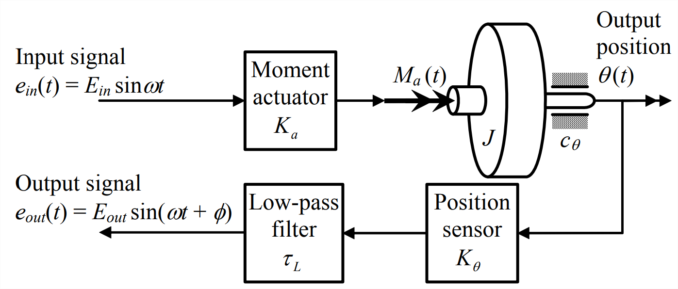
The observation that, for \(\Lambda=\Lambda_{n s}\), output \(e_{\text {out}}(t)=-E_{i n} \sin \omega_{n s} t\) in response to input \(e_{i n}(t)=E_{i n} \sin \omega_{n s} t\) provides motivation for conducting steady-state-sinusoidal tests on the open-loop system over a band of frequencies surrounding \(\omega_{n s}\), not just \(\omega_{n s}\), and for other values of \(\Lambda\), not just \(\Lambda_{n s}\), in order determine if this type of testing provides information regarding the stability of the closed-loop system. We can simulate such a test by evaluating numerically the open-loop frequency-response function, from Equation \(\ref{eqn:17.2}\):

\[O L F R F(\omega) \equiv O L T F(j \omega)=\Lambda \frac{\omega_{b}}{j \omega\left(j \omega+c_{\theta} / J\right)\left(j \omega+\omega_{b}\right)}\label{eqn:17.5} \]

To begin, in order to establish a reference set of results for the neutral-stability value of gain, \(\Lambda=\Lambda_{n s}\), we calculate and plot from Equation \(\ref{eqn:17.5}\) frequency-response components using the following MATLAB code:

>> wb=300;coj=100;wns=sqrt(wb*coj);

>> wbar=logspace(-1,1,100);w=wbar*wns;

>> lm=4e4;olfrf4e4=lm*wb./(j*w.*(j*w+coj).*(j*w+wb));

>> subplot(2,1,1),loglog(wbar,abs(olfrf4e4)),grid

>> faz=atan(imag(olfrf4e4)./real(olfrf4e4))-pi*ones(1,length(w));

>> subplot(2,1,2),semilogx(wbar,faz*180/pi),grid

Figure \(\PageIndex{3}\) includes the graphical results from these MATLAB operations. For now, we focus on just the plots of the polar components, magnitude ratio and phase angle, for \(\Lambda=\Lambda_{n s}=40,000\) s^-2; the additional annotations on the phase plot for “PM” at other values of \(\Lambda\) will be explained in due course. If we were testing the real hardware of Figure \(\PageIndex{2}\), rather than just numerically simulating a test, then the magnitude ratio would be the measured quantity \(E_{\text {out}} / E_{\text {in}}\) as frequency \(\omega\) is varied, and the phase angle \(\phi\) would be calculated from measurements by the method presented in Section 4.4.

Figure \(\PageIndex{3}\): Modified Bode diagram, Equation \(\ref{eqn:17.5}\), frequency response for \(\Lambda=\Lambda_{n s}= 40,000\) s^-2 of the open-loop system in Figure \(\PageIndex{2}\) (Copyright; author via source)

Figure \(\PageIndex{4}\): Magnitude ratios, Equation \(\ref{eqn:17.5}\) for \(\Lambda = 4,000\) and \(400,000\) s^-2. (Copyright; author via source)

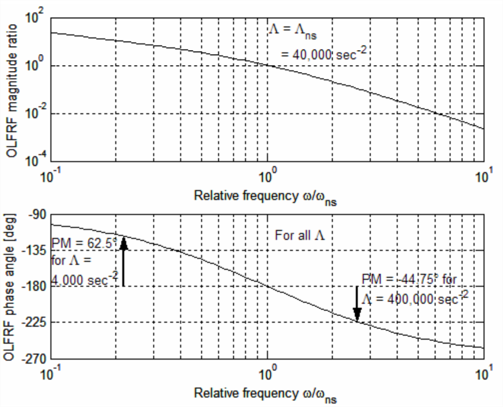
The upper plot of Figure \(\PageIndex{3}\) shows that, for \(\Lambda=\Lambda_{n s}\), magnitude ratio \(|O L F R F|\) varies smoothly from greater than 10 at \(\omega=0.1 \omega_{n s}\), through the previously determined value of 1 at \(\omega=\omega_{n s}\), down to less than 0.01 at \(\omega=10 \omega_{n s}\). The lower plot shows that phase angle \(\angle O L F R F\) is a lag ranging from more than −90° at \(\omega=0.1 \omega_{n s}\), through the previously determined phase of −180° at \(\omega=\omega_{n s}\), down to a lag approaching −270° at \(\omega=10\omega_{n s}\). We have from Equation \(\ref{eqn:17.4}\) for \(\Lambda=\Lambda_{n s}\), \(\angle O L F R F\left(\omega_{n s}\right)=(\pm \pi, \pm 3 \pi, \ldots)\), which is ambiguous regarding the multiple and sign of \(\pi\) that is appropriate; the phase plot of Figure \(\PageIndex{3}\) removes the ambiguity, at least for this system: clearly, \(\angle O L F R F\left(\omega_{n s}\right)=-\pi\) rad.²

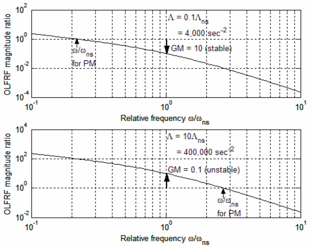
With Figure \(\PageIndex{3}\) for \(\Lambda=\Lambda_{n s}\) as the reference open-loop frequency response representing the neutrally stable closed-loop system, we can now compute simulated open-loop frequency responses for other values of \(\Lambda\), specifically, those for which the closed-loop system is oscillatory and either exponentially stable or unstable. With the following MATLAB code, we calculate and plot on Figure \(\PageIndex{4}\) (on the previous page) the magnitude-ratio (only) frequency-response graphs for the gain \(\Lambda=0.1 \Lambda_{n s}=4,000\) s^-2, for which we know the closed-loop system is stable, and for the gain \(\Lambda=10 \Lambda_{n s}=400,000\) s^-2, for which we know the closed-loop system is unstable:

>> wb=300;coj=100;wd=sqrt(wb*coj);

>> wbar=logspace(-1,1,100);w=wbar*wd;

>> lm=4e3;olfrf4e3=lm*wb./(j*w.*(j*w+coj).*(j*w+wb));

>> lm=4e5;olfrf4e5=lm*wb./(j*w.*(j*w+coj).*(j*w+wb));

>> subplot(2,1,1),loglog(wbar,abs(olfrf4e3)),grid

>> subplot(2,1,2),loglog(wbar,abs(olfrf4e5)),grid

If we were to calculate the phase angles for any value of \(\Lambda\), we would find them to be identical to those on the phase-angle graph for \(\Lambda=\Lambda_{n s}\) of Figure \(\PageIndex{3}\), which is the reason for not repeating the phase-angle calculations. (The theory behind this feature of openloop phase angle, and also the variation of open-loop magnitude for different values of \(\Lambda\), will be presented at the end of this section.)

By comparing the open-loop magnitude-ratio graphs of Figures \(\PageIndex{3}\) and \(\PageIndex{4}\), we observe the magnitudes for the closed-loop stable case \(\Lambda=0.1 \Lambda_{n s}\) to be less than those for neutral stability, \(\Lambda=\Lambda_{n s}\), and the magnitudes for the unstable case \(\Lambda=10 \Lambda_{n s}\) to be greater. We conclude from this that open-loop magnitudes less than or greater than those for neutral stability are an indication of closed-loop absolute stability. If we were to calculate the open-loop magnitude ratios for other values between \(0.1 \Lambda_{n s}\) and \(10 \Lambda_{n s}\), we would find that the variation is monotonic and regular; this suggests that open-loop magnitude can also provide a metric for closed-loop relative stability, i.e., the degree of stability or instability. Indeed, there is a commonly accepted metric called gain margin (\(\text { GM }\)); if we denote the gain margin for a particular value of \(\Lambda\) as \(\operatorname{GM}(\Lambda)\), then it is defined as the following dimensionless ratio of open-loop magnitudes:

\[\operatorname{GM}(\Lambda) \equiv \frac{\left|O L F R F\left(\omega_{n s}\right)\right|_{\Lambda_{n s}} \mid \text { at }\left.\angle O L F R F\left(\omega_{n s}\right)\right|_{\Lambda_{n s}}=-180^{\circ}}{|O L F R F(\omega)|_{\Lambda} \mid \text { at }\left.\angle O L F R F(\omega)\right|_{\Lambda}=-180^{\circ}}=\frac{1}{|O L F R F(\omega)|_{\Lambda} \mid \text { at }\left.\angle O L F R F(\omega)\right|_{\Lambda}=-180^{\circ}}\label{eqn:17.6} \]

In the second form of Equation \(\ref{eqn:17.6}\), which is the working definition, we applied the unit magnitude value derived in Equation \(\ref{eqn:17.4}\). The condition \(\left.\angle O L F R F(\omega)\right|_{\Lambda}=-180^{\circ}\) is called, descriptively, a phase crossover.

Applying Equation \(\ref{eqn:17.6}\) to Figures \(\PageIndex{3}\) and \(\PageIndex{4}\), we calculate these gain margins: \(\mathrm{GM}\left(0.1 \Lambda_{n s}\right)=10\) for the closed-loop stable system; and \(\operatorname{GM}\left(10 \Lambda_{n s}\right)=0.1\) for the unstable system. Clearly, \(\mathrm{GM}>1\) implies closed-loop stability and \(0<\mathrm{GM}<1\) implies instability. Expressing \(\text { GM }\) in terms of its logarithm to the base 10 (denoted “log”) is also of value, since in this form \(\text { GM }\) is positive for closed-loop stability, zero for neutral stability, and negative for instability. It is traditional in control-system engineering to express \(\text { GM }\) in decibels (dB), in which unit the value of a positive number \(N\) is \(20 \times \log N\) dB. Accordingly, \(\operatorname{GM}\left(0.1 \Lambda_{n s}\right)=+20\) dB for the closed-loop stable case of Figure \(\PageIndex{4}\), and \(\operatorname{GM}\left(10 \Lambda_{n s}\right)=-20\) dB for the unstable case.

Another open-loop frequency-response metric for closed-loop degree of stability is the phase margin (PM). The phase margin for a given value \(\Lambda\) of the control parameter is defined as the lag angle at the frequency for which the magnitude ratio is unity relative to the comparable lag angle for the neutral-stability case, \(\Lambda=\Lambda_{n s}\):

\[\operatorname{PM}(\Lambda)=\left(\left.\angle O L F R F(\omega)\right|_{\Lambda} \text { at }|O L F R F(\omega)|_{\Lambda} \mid=1\right)-\left(\left.\angle O L F R F\left(\omega_{n s}\right)\right|_{\Lambda_{n s}} \text { at }\left|O L F R F\left(\omega_{n s}\right)\right|_{\Lambda_{n s}} \mid=1\right) \nonumber \]

From Equation \(\ref{eqn:17.4}\) and the phase plot of Figure \(\PageIndex{3}\), the reference lag angle is just −180°, so

\[\operatorname{PM}(\Lambda)=180^{\circ}+\left(\left.\angle O L F R F(\omega)\right|_{\Lambda} \text { at }|O L F R F(\omega)|_{\Lambda} \mid=1\right)\label{eqn:17.7} \]

The condition \(|O L F R F(\omega)|_{\Lambda} \mid=1\) is called a gain crossover. Reading approximately the appropriate phases from the phase plot of Figure \(\PageIndex{3}\), we calculate these phase margins: \(\operatorname{PM}\left(0.1 \Lambda_{n s}\right) \approx 180^{\circ}-120^{\circ}=+60^{\circ}\) for the closed-loop stable system, and \(\operatorname{PM}\left(10 \Lambda_{n s}\right) \approx 180^{\circ}-225^{\circ}=-45^{\circ}\) for the unstable system. (See homework Problem 17.2(a) for calculation of the more precise values of \(\mathrm{PM}\) annotated on Figure \(\PageIndex{3}\).) Clearly, \(\mathrm{PM}>0^{\circ}\) implies closed-loop stability and \(\mathrm{PM}<0^{\circ}\) implies instability.

Brogan, 1974, page 25, described succinctly the practical interpretation of these stability margins for an initially stable closed-loop system: “Gain margin \(\text { GM }\) is a measure of additional gain a system can tolerate with no change in phase, while remaining stable. Phase margin \(\mathrm{PM}\) is the additional phase shift that can be tolerated, with no gain change, while remaining stable.”

We have defined and illustrated gain and phase margins for stable and unstable feedback control using the physical system of Figures 16.3.1, 16.3.2, and \(\PageIndex{2}\). The behavior of this physical system is fairly “common” in the sense that it is stable for gain \(\Lambda=0\) and for low positive values of \(\Lambda\), but it is unstable for all values of \(\Lambda\) greater than a particular neutral-stability value, \(\Lambda_{n s}\). For any such common physical system, the open-loop frequency-response metrics of gain margin and phase margin described in this section are valid measures of absolute and relative stability. However, for “uncommon” physical systems, gain margins and phase margins of open-loop frequency response can be ambiguous and difficult to interpret; for example, such an uncommon system might have \(\mathrm{PM}=+78^{\circ}\) but \(\mathrm{GM}=-10\) dB, yet still be closed-loop stable. For such uncommon systems, a more general and involved, but unambiguous, approach to frequency-response analysis is based on the Nyquist stability criterion, which is the subject of Section 17.3.

Now that we know how to calculate open-loop frequency responses in the format of Figures \(\PageIndex{3}\) and \(\PageIndex{4}\) using standard MATLAB commands, it is appropriate that we not have to do so for every problem, but, instead, that we can apply the built-in MATLAB functions margin and bode to produce more easily the same results. Before calling one of these functions, it is necessary first to define with the tf command a MATLAB lineartime-invariant (LTI) transfer-function model. The following, for the gain \(\Lambda=10 \Lambda_{n s}\) of the same system as that of Figures \(\PageIndex{3}\) and \(\PageIndex{4}\), shows one of the many ways to do this, along with the MATLAB responses:

>> wb=300;coj=100;

>> s=tf('s')

Transfer function:

s

>> lm=4e5;oltf4e5=lm*wb/(s*(s+coj)*(s+wb))

Transfer function:

1.2e008

----------------------- s^3 + 400 s^2 + 30000 s

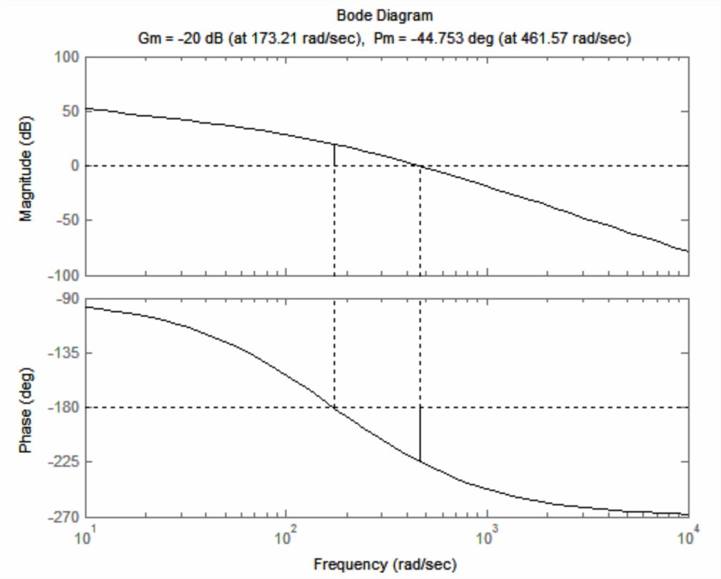
>> margin(oltf4e5)

This margin command produced the Bode diagram or plot of Figure \(\PageIndex{5}\) (next page), which is annotated with the \(\mathrm{GM}\) and \(\mathrm{PM}\) for this case, \(\Lambda=10 \Lambda_{n s}\), that of the unstable closed-loop system. (The bode function itself also produces the Bode diagram, but without calculating and printing the \(\mathrm{GM}\) and \(\mathrm{PM}\).) Note that it was not necessary to specify the frequency band—MATLAB chose an appropriate band. By comparing Figure \(\PageIndex{5}\) with Figures \(\PageIndex{3}\) and \(\PageIndex{4}\), you should observe some differences in format, which is why Figure \(\PageIndex{3}\) is labeled a “modified” Bode diagram; but there are no differences in the essential content. A traditional Bode diagram such as Figure \(\PageIndex{5}\) plots the frequency-response magnitude ratio (in decibels) versus frequency (in rad/s or Hz), which is presented on a logarithmic scale in order to accommodate a very wide band.

Figure \(\PageIndex{5}\): MATLAB’s traditional Bode diagram, Equation \(\ref{eqn:17.5}\), frequency response for \(\Lambda=10 \Lambda_{n s}=400,000\) s^-2 of the open-loop system in Figure \(\PageIndex{2}\). (Copyright; author via source)

To conclude this section, we consider for systems in general how changes in gain \(\Lambda\) influence open-loop frequency responses and their graphical representations on Bode diagrams (and Nyquist diagrams in Section 17.4). We infer from Equations 16.6.2 and 16.6.3 that an open-loop transfer function can generally be expressed in the form

\[\operatorname{OLTF}(s)=\Lambda \times T F_{1}(s)\label{eqn:17.8} \]

where the baseline transfer function \(T F_{1}(s)\) is obviously defined as \(\left.O L T F(s)\right|_{\Lambda=1}\). The associated general frequency-response function is

\[O L F R F(\omega)=\Lambda \times T F_{1}(j \omega)=\Lambda \times\left|T F_{1}(j \omega)\right| \times \exp \left[j \angle T F_{1}(j \omega)\right]\label{eqn:17.9} \]

Equation \(\ref{eqn:17.9}\) leads to the following general forms for open-loop frequency-response magnitude ratio (\(\mathrm{MR}\)) and phase angle \(\phi\):

\[M R(\omega)=|O L F R F(\omega)|=\Lambda \times\left|T F_{1}(j \omega)\right| \equiv \Lambda \times M R_{1}(\omega)\label{eqn:17.10} \]

\[\phi(\omega)=\angle T F_{1}(j \omega)\label{eqn:17.11} \]

Equation \(\ref{eqn:17.11}\) shows that the variation of phase angle with frequency, \(\phi(\omega)\), is the same for all values of gain \(\Lambda\), as was stated earlier in the context of Figures \(\PageIndex{3}\) and \(\PageIndex{4}\).

In the final form of Equation \(\ref{eqn:17.10}\), we define the baseline magnitude ratio (i.e., for unity gain, \(\Lambda=1\)) as \(M R_{1}(\omega) \equiv\left|T F_{1}(j \omega)\right|\). It is also informative to express Equation \(\ref{eqn:17.10}\) in a logarithmic form, either in logarithm to base 10 as on Figures \(\PageIndex{3}\) and \(\PageIndex{4}\), or in decibels as on a traditional Bode plot such as Figure \(\PageIndex{5}\):

\[\log (M R(\omega))=\log (\Lambda)+\log \left(M R_{1}(\omega)\right)\label{eqn:17.12a} \]

\[20 \times \log (M R(\omega)) \equiv[M R(\omega)](\mathrm{dB})=[\Lambda](\mathrm{dB})+\left[M R_{1}(\omega)\right](\mathrm{dB})\label{eqn:17.12b} \]

We infer from Equations \(\ref{eqn:17.10}\), \(\ref{eqn:17.12a}\), and \(\ref{eqn:17.12b}\) that the graphical shape of the functional variation with frequency of magnitude ratio \(M R(\omega)\) does not change with changes in gain \(\Lambda\). For modified Bode plots such as Figures \(\PageIndex{3}\) and \(\PageIndex{4}\), given the baseline curve \(M R_{1}(\omega)\), we can find from Equation \(\ref{eqn:17.12a}\) the curve for any other gain \(\Lambda>1\) just by adding to the baseline curve the value \(\log (\Lambda)\), which moves the entire curve up by the distance \(\log (\Lambda)\) along the magnitude-ratio axis. The process of finding curves for different gains \(\Lambda\) from Equation \(\ref{eqn:17.12b}\) is easy for a traditional Bode plot such as Figure \(\PageIndex{5}\), on which magnitude is plotted in decibels with a linear scale. For example, we can find from Figure \(\PageIndex{5}\) the magnitude curve for \(\Lambda=40,000\) s^-2 simply by moving downward by 20 dB, i.e., by \(20 \times [\log (40,000)-\log (400,000)]\), the magnitude curve for \(\Lambda=400,000\) s^-2.

¹We use the Laplace complex variable \(s\) in this chapter because it is traditional for treatment of frequency-response theory to use \(s\), instead of complex variable \(p\) (for \(s = p\), a solution of the characteristic equation, i.e., a pole of the closed-loop transfer function) that we used in Sections 16.3 through 16.6.

²The line of MATLAB code that calculates phase requires the angles to be between \(-\pi / 2\) and \(-3\pi / 2\) rad, so the argument here appears to be circular. However, if we were to use the more general MATLAB function angle in place of that line of code, we would find, in the range of \(0.1 \leq \omega / \omega_{n s}<1.0\), exactly the same lagging phases as are on the phase plot of Figure \(\PageIndex{3}\), which does validate the assertion that the appropriate value is \(-\pi\) rad. We did not use angle, because it is apparently based upon MATLAB’s four-quadrant inverse tangent functionatan2, which returns angle values only between \(-\pi\) and \(+\pi\) rad. Therefore, on the graph of phase versus \(\omega / \omega_{n s}\), angle would produce an artificial and confusing discontinuous jump in phase from −180° to +180° at \(\omega / \omega_{n s}=1.0\) and, in the range of \(1.0 \leq \omega / \omega_{n s} \leq 10\), phase would drop from +180° to a little more than +90°.