17.2: Nyquist Plots

We now depart temporarily from the analysis of stability in order to describe a type of frequency-response graphical representation that has not appeared previously in this book. Such a graph is commonly called, in the language of control-system engineering, a Nyquist diagram or plot.

We begin the description of Nyquist plots by re-visiting a familiar system from several previous chapters: the standard, positively damped 2^nd order system. The ODE of this system for output \(x(t)\) in response to input \(u(t)\) is \(\ddot{x}+2 \zeta \omega_{n} \dot{x}+\omega_{n}^{2} x=\omega_{n}^{2} u(t)\) [Equation 9.2.2], and the frequency-response function is

\[F R F(\omega)=\frac{\omega_{n}^{2}}{\omega_{n}^{2}-\omega^{2}+j 2 \zeta \omega_{n} \omega}\label{eqn:10.7} \]

The previous graphical representation of Equation \(\ref{eqn:10.7}\) in this book is Figure 10.2.1, a modified Bode diagram displaying the variation with frequency \(\omega\) of the polar components, magnitude ratio \(|F R F(\omega)|\) and phase angle \(\phi=\angle F R F(\omega)\). A Nyquist plot, in contrast, displays directly the mathematical rectangular components, in the format \(\operatorname{Im}[F R F(\omega)]\) versus \(\operatorname{Re}[F R F(\omega)]\), with frequency \(\omega\) being the implicit independent variable, for which there is no graduated scale without extra annotation or a three-dimensional third axis perpendicular to the complex \(F R F(\omega)\)-plane. For example, the following MATLAB commands produce Figure \(\PageIndex{1}\), a Nyquist plot of Equation \(\ref{eqn:10.7}\) for undamped natural frequency \(\omega_{n} = 2\pi\) rad/s and damping ratio \(\zeta=0.2\):

>> wn=2*pi;zt=0.2;

>> w=wn*logspace(-2,2,400);

>> frf=wn^2./(wn^2-w.^2+j*2*zt*wn*w);

>> plot(real(frf),imag(frf)),grid

Figure \(\PageIndex{1}\): Nyquist plot of \(F R F(\omega)=\omega_{n}^{2} /\left(\omega_{n}^{2}-\omega^{2}+j 2 \zeta \omega_{n} \omega\right)\) for \(\omega_{n}=2 \pi\) rad/s and \(\zeta=0.2\). (Copyright; author via source)

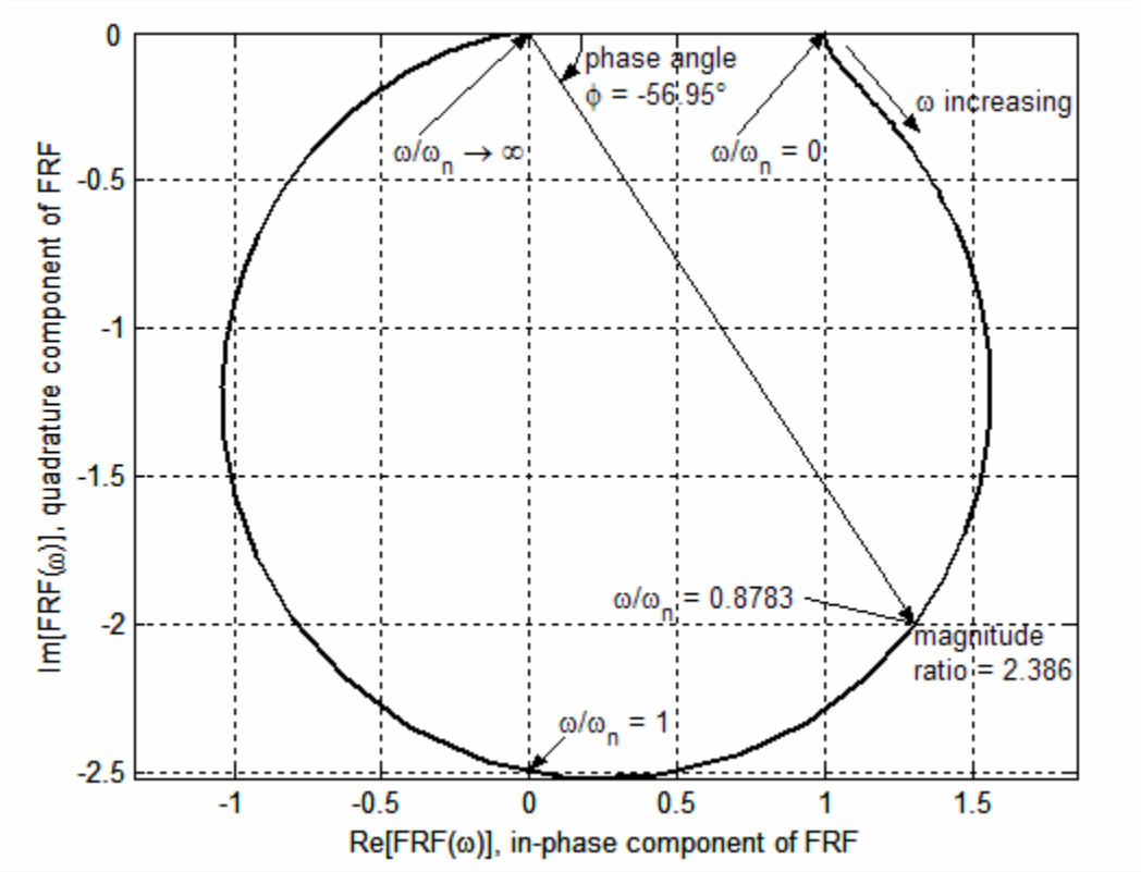
Observe on Figure \(\PageIndex{1}\) that the abscissa and ordinate axes are labeled both with the mathematical descriptions, \(\operatorname{Re}[F R F(\omega)]\) and \(\operatorname{Im}[F R F(\omega)]), and with the corresponding physical descriptions of the response components, respectively: in-phase (0°, also known as coincident) and quadrature (leading by 90°). If you were measuring frequency response experimentally on a damped 2^nd order system you might generate the physical information of Figure \(\PageIndex{1}\) in the following manner: first, measure the polar components of response, magnitude ratio \(|F R F(\omega)|\) and phase angle \(\phi(\omega)=\angle F R F(\omega)\), using the procedure described in Section 17.1 relative to Figure 17.1.3, the modified Bode diagram; then, use Equation 2.1.7 for converting complex numbers from polar form into rectangular form to calculate \(F R F_{\text {in-phase}}(\omega)=|F R F(\omega)| \times \cos \phi(\omega)\) and \(F R F_{\text {quadrature}}(\omega)=|F R F(\omega)| \times \sin \phi(\omega)\). An example of this conversion is illustrated on Figure \(\PageIndex{1}\) for \(\omega=0.8783 \omega_{n}\): \(1.301 = 2.386 \times \cos \left(-56.95^{\circ}\right)\), and \(-2.000=2.386 \times \sin \left(-56.95^{\circ}\right)\).

The concept of physical in-phase and quadrature frequency-response components might seem strange. Moreover, their values can be either positive or negative (as Figure \(\PageIndex{1}\) shows for the in-phase component), and that might be confusing: if a pure “in-phase” response is negative, then the response is actually 180° out of phase with the excitation; and if a pure “quadrature” response is negative, then the response actually lags the excitation by 90°. In order to provide more clarity, even at the risk of being redundant, we present the following table, which lists multiple-of-90° values of phase angle \(\phi\) that correspond to particular values or ranges of the in-phase and quadrature components.

In-phase Component	Quadrature component	Phase angle \(\phi\)
\(>0\)	\(=0\)	\(0^{\circ} \text { and } \mp 360^{\circ}\)
\(=0\)	\(<0\)	\(-90^{\circ} \text { and }+270^{\circ}\)
\(<0\)	\(=0\)	\(\mp 180^{\circ}\)
\(=0\)	\(>0\)	\(-270^{\circ} \text { and }+90^{\circ}\)

It might be instructive also to compare the Nyquist plot of Figure \(\PageIndex{1}\) with the corresponding polar components for \(\zeta=0.2\) on the modified Bode plots of Figure 10.2.1. On both figures for \(\omega \approx 0\), the response is essentially the static value, \(F R F(0)=+1+j 0\). As frequency \(\omega\) increases from \(0+\) to \(\omega_n\), the magnitude ratio varies (mostly increasing) from +1 to \(1 /(2 \zeta)=2.5\), while the phase angle, a lag, varies from 0° to −90°. At \(\omega=\omega_{n}\), the response is pure negative quadrature, \(F R F\left(\omega_{n}\right)=0-j 2.5\). As \(\omega\) increases above \(\omega_n\), the magnitude ratio decreases monotonically while the phase lags further, with the magnitude ratio approaching zero and the phase approaching −180° as \(\omega \rightarrow \infty\).

Frequency response of the standard, positively damped 2^nd order system is well behaved, especially for \(\omega = 0\), i.e., a non-zero input that is constant in time, for which the system has an unquestionably stable non-zero constant static output. Let us consider now Nyquist plotting for a contrasting system, an open-loop system that lacks a stable static response, the system of Section 17.1 (also Sections 16.3, 16.5, and 16.6). The clearest indication of a possible difficulty is Equation 17.1.7 for \(\operatorname{OLFRF}(\omega)\), which indicates an infinite response for \(\omega = 0\). The mathematical source of this difficulty is the pole of \(O \operatorname{LTF}(s)\) at the \(s\)-plane origin, which is apparent in Equation 17.1.2, Figure 16.6.2, and elsewhere. The graphical display of frequency response magnitude becoming very large as \(\omega \rightarrow 0\) is produced by the following MATLAB commands, which calculate frequency response and produce a Nyquist plot of the same numerical solution as that on Figure 17.1.3, for the neutral-stability case \(\Lambda=\Lambda_{n s}=40,000\) s^-2:

>> wb=300;coj=100;wns=sqrt(wb*coj);

>> wbar=logspace(-1,1,200);w=wbar*wns;

>> lm=4e4;olfrf4e4=lm*wb./(j*w.*(j*w+coj).*(j*w+wb));

>> plot(real(olfrf4e4),imag(olfrf4e4)),grid

Figure \(\PageIndex{2}\) is an annotated portion of the MATLAB graph that displays the noteworthy features of the Nyquist plot. This plot shows that for frequency \(\omega\) becoming progressively smaller, the negative quadrature component of response becomes progressively larger.

Figure \(\PageIndex{2}\): Nyquist plot, Equation 17.1.7, frequency response for \(\Lambda=\Lambda_{n s}=40,000\) s^-2 of the open-loop system in Figure 17.1.2, with parameters \(\omega_{b}=300\) s^-1, \(c_{\theta} / J=100\) s^-1, and \(\omega_{n s}=\sqrt{\omega_{b} \times c_{\theta} / J}=173.2\) rad/s. (Copyright; author via source)

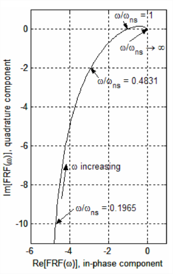
In fact, we can calculate from Equation 17.1.7 the asymptotic nature of the variation of open-loop frequency response as \(\omega \rightarrow 0\), by applying the method of complex rectangular division described in Section 2.1:

\[O L F R F(\omega)=\frac{\Lambda \omega_{b}}{j \omega\left(j \omega+c_{\theta} / J\right)\left(j \omega+\omega_{b}\right)}=\frac{40,000 \times 300}{(j \omega)^{3}-(100+300) \omega^{2}+(100 \times 300) j \omega}=\frac{1.2 \times 10^{7} \times\left[-400 \omega^{2}-j\left(3 \times 10^{4} \omega-\omega^{3}\right)\right]}{9 \times 10^{8} \omega^{2}+1 \times 10^{5} \omega^{4}+\omega^{6}} \nonumber \]

Therefore, as \(\omega \rightarrow 0\),

\[\operatorname{OLFRF}(\omega) \rightarrow \frac{1.2 \times 10^{7} \times\left[-400 \omega^{2}-j\left(3 \times 10^{4} \omega\right)\right]}{9 \times 10^{8} \omega^{2}}=-51 / 3-j \frac{400}{\omega}\label{eqn:17.13} \]