1.1: MATLAB Basics

Learning Objectives

By the end of this lab, students will be able to:

1. Get help and documentation for MATLAB functions
2. Solve matrix-vector equations in MATLAB
3. Manipulate complex numbers in MATLAB
4. Vectorize a simple equation
5. Use MATLAB’s plotting tools to graph signals

This lab will also preview future labs by demonstrating how to play audio signals and display images.

Overview

This lab introduces the MATLAB computing environment. MATLAB is an extremely useful tool for signals and systems as well as for many other computing tasks. Unlike C, C++, or Java, there is no need to compile MATLAB code, making debugging and experimenting much easier. The purpose of this lab is not to provide a comprehensive introduction to MATLAB, but to help students get comfortable enough to learn more on their own. Future labs will introduce new MATLAB content as necessary.

Note: Most of this lab was developed using MATLAB versions R2017b and R2019a. Compatibility across versions is generally very good in MATLAB, but the appearance of the GUIs tends to change.

Pre-Lab Reading

MATLAB is a commercial software product produced by MathWorks. The software includes both a numeric computing environment and a programming language, though “MATLAB” often refers to the programming language. MATLAB is commonplace in industry and academia. You will benefit from understanding the basics of using MATLAB.

Many university students can obtain student versions of MATLAB for free. Instructions for Iowa State University students can be found here: https://it.engineering.iastate.edu/how-to/installing-matlab/. Free alternatives to MATLAB include GNU Octave (https://www.gnu.org/software/octave/), Scilab (https://www.scilab.org/), and FreeMat(http://freemat.sourceforge.net/).

MATLAB stands for “MATrix LABoratory,” as it was first developed to allow university students to easily use numeric computing software for linear algebra. Part of what makes MATLAB easy to use is that there is no need to compile MATLAB code before running it. Code can be entered and executed line by line in the Command Window. Reflecting its roots in linear algebra¹, all variables are essentially matrices by default. Variables do not have to be declared before they are used, and usually it is unnecessary to specify the class of a variable. These factors make it easy to get started in MATLAB, though they can be disorienting for those used to compiled languages like C, C++, and Java.

Lab Exercises

Getting Started

Figure \(\PageIndex{1}\): The MATLAB Desktop

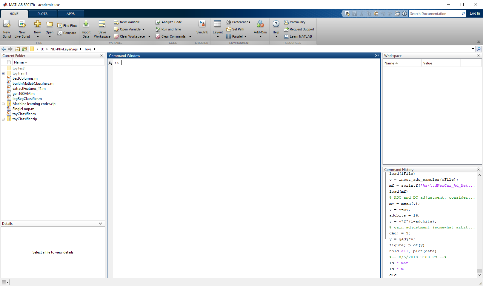
Upon starting up MATLAB, you will see the MATLAB Desktop (see Figure \(\PageIndex{1}\)) which consists of the Tool Strip, Current Folder window, Command Window, Workspace, and Command History. The purpose of these windows is largely self-explanatory, but we will touch on them occasionally as necessary. Perhaps the best way to jump into MATLAB is to learn how to get help. You can simply type help followed by the name of a function to get help on that function. You can even get help for the function help:

>> help help

Another great way to get help is with the doc command. Whereas help gives you a (usually) brief explanation in the Command Window, doc opens up more thorough documentation in a new window. Use the doc command to find out about the many ways to use the colon (:) in MATLAB:

>> doc colon

MATLAB also has built in demos to help you use various functions and tools. You can type help demo to learn about how to run the examples, or you can just type demo to open up a new window with featured examples. Find and click on the “Basic Matrix Operations” demo. This will display the demo in the help window. Click the “Open Live Script” button in the upper right. This will open the demo as a live script in MATLAB’s Live Editor. Step through the live script by clicking the “Run Section” or “Run and Advance” buttons in the Live Editor’s Tool Strip. Make sure you understand what is happening with each command. (Most of you probably don’t know what it means to “convolve” two vectors yet, but you will in a few weeks!)

Solving Systems of Linear Equations

Figure \(\PageIndex{2}\): A simple circuit

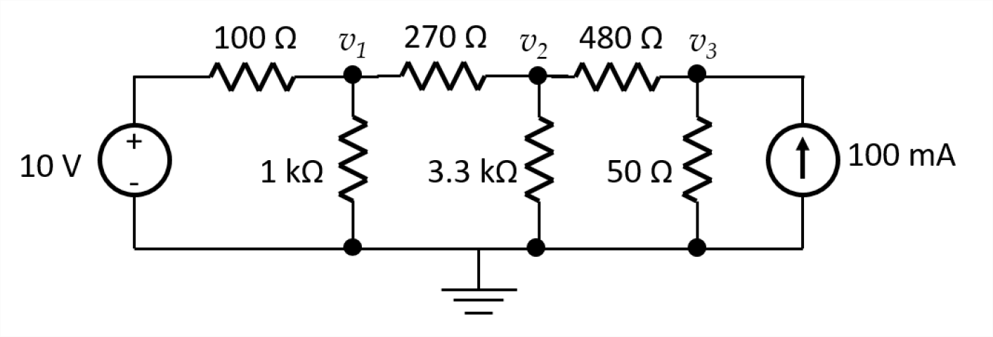
Now that you have seen an example of solving a matrix equation \(\mathbf{y} = \mathbf{H} \mathbf{x}\) for \(\mathbf{x}\), let’s apply this to something you know. Consider the circuit shown in Figure \(\PageIndex{2}\). In EE 201, you learned that the voltages \(v_1\), \(v_2\), and \(v_3\) in this circuit can be found via the Node Voltage Method. Assuming you remember how to do that, you will arrive at the following set of equations: \[\begin{aligned} \frac{v_1 -10}{100} + \frac{v_1}{1000} + \frac{v_1 - v_2}{270} &= 0 \\ \frac{v_2 - v_1}{270} + \frac{v_2}{3300} + \frac{v_2 - v_3}{480} &= 0 \\ \frac{v_3 - v_2}{480} + \frac{v_3}{50} &= 0.1\end{aligned} \nonumber \] We can rewrite these as a matrix vector equation: \[\begin{aligned} \begin{bmatrix} \frac{1}{100}+\frac{1}{1000}+\frac{1}{270} & \frac{-1}{270} & 0 \\ \frac{-1}{270} & \frac{1}{270}+\frac{1}{3300}+\frac{1}{480} & \frac{-1}{480} \\ 0 & \frac{-1}{480} & \frac{1}{480}+\frac{1}{50} \end{bmatrix} \begin{bmatrix} v_1 \\ v_2 \\ v_3 \end{bmatrix} &= \begin{bmatrix} \frac{10}{100} \\ 0 \\ 0.1 \end{bmatrix}\end{aligned} \nonumber \] Use MATLAB to solve for the voltages \(v_1\), \(v_2\), and \(v_3\). Be sure to include the code you used in your lab report.

HINT: You can use the diary function to keep track of the commands you use in MATLAB. Type help diary to find out how.

Complex Numbers in MATLAB

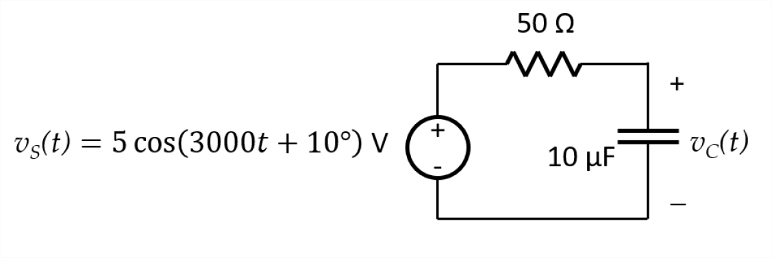
Consider the A/C circuit shown in Figure \(\PageIndex{3}\). Recall that the steady-state response of this circuit can be found using phasors. In the phasor domain, we can use a voltage divider to find the phasor voltage on the capacitor: \(\mathbf{V}_C = \frac{-j \frac{100}{3}}{50 - j \frac{100}{3}} 5\angle{10^\circ}\). Rearranging and recalling that the phasor notation \(5\angle{10^\circ}\) means \(5 e^{j 10 \frac{\pi}{180}}\), we have: \[\begin{aligned} \mathbf{V}_C &= \frac{1}{j 1.5 + 1 } 5 e^{j \frac{\pi}{18}} \label{eq:phasor}\end{aligned} \] Let’s use MATLAB to find \(\mathbf{V}_C\).

Figure \(\PageIndex{3}\): An RC circuit

MATLAB naturally handles complex numbers and complex arithmetic. There are several ways to represent the imaginary unit (\(\sqrt{-1}\)). Try typing the following in MATLAB.

>> a = i;
>> b = j;
>> c = 1i;
>> d = 1j;
>> a, b, c, d

You should see that MATLAB displays the value of each variable as 0.0000 + 1.0000i. You can check that this is indeed \(\sqrt{-1}\) by using the equality operator “==”:

>> a == sqrt(-1)

Notice the difference between assignment (=) and equality (==).

Now we can solve Equation [eq:phasor] in MATLAB. Rather than just typing in the right-hand side of the equation, we will use variables for each quantity:

>> om = 3000; C = 1e-5; R = 50;
>> Vs = 5*exp(1i*10*pi/180);
>> Zc = -1i/om/C;
>> Zr = R;
>> Vc = Zc/(Zr+Zc)*Vs

MATLAB should display an answer of 1.9158 - 2.0055i. Before we explore what that means, there are a few important things to notice about MATLAB in these lines. First, we can type lots of commands on one line; separating by a semicolon (;) stops MATLAB from displaying the result of each. (Try using a comma (,) instead.) Second, angles in MATLAB are assumed to be in radians, so we converted \(10^\circ\) to \(10\pi/180\) radians. Third, the number \(\pi\) is built in to MATLAB. Other built-in values include infinity (inf), not-a-number (NaN), and the output of the last command (ans)². Fourth, MATLAB uses order of operations the way most scientific calculators and other programming languages do. You can find out exactly how MATLAB orders operations by typing “operator precedence” in the search bar in the upper right corner of the MATLAB desktop.

Using MATLAB we found that \(\mathbf{V}_C = 1.9158 - 2.0055i\) V; however, we would like to have the answer in phaser form. In MATLAB we can use abs and angle to convert \(\mathbf{V}_C\) to polar form or phasor form. Try it yourself. Once you have the magnitude and phase of the capacitor voltage, find the time-domain voltage, \(v_C(t)\), and record this in your lab report. Remember to use a degree sign (\(^\circ\)) if you choose to report the phase angle in degrees.

There are a few other commands that are useful when working with complex numbers. You can type real(Vc) or imag(Vc) to get ther real or imaginary parts of Vc. conj(Vc) returns the complex conjugate of Vc.

>> real(Vc)

ans =

    1.9158

>> imag(Vc)

ans =

   -2.0055

>> conj(Vc)

ans =

   1.9158 + 2.055i

Vectorization

MATLAB is optimized for operations involving matrices and vectors. For example, we could use the following code to multiply matrices \(\mathbf{A}\) and \(\mathbf{B}\) and store the result in matrix \(\mathbf{C}\) (assuming \(\mathbf{C}\) has been initialized to all zeros):

>> for x = 1:size(A,1)
>>     for y = 1:size(B,2)
>>         for z = 1:size(A,2)
>>             C(x,y) = C(x,y) + A(x,z) * B(z,y);
>>         end
>>     end
>> end

Not ony is this annoying to type, but it also executes less efficiently than simply typing:

>> C = A*B;

Likewise, matrix-vector products can be found by typing y = H*x for matrix \(\mathbf{H}\) and vectors \(\mathbf{x}\) and \(\mathbf{y}\). We can multiply matrices or vectors by scalars by simply typing a*H or a*y. Almost all MATLAB operations are designed to be applied to matrices. In fact, it is good programming practice to avoid for loops in MATLAB (though sometimes they are unavoidable).

Let’s use vectorization to our advantage. Suppose we want to know the steady-state output voltage \(\mathbf{V}_C\) for the circuit in Figure 3 for the following input voltages:

• \(v_S(t) = 5 \cos{(3000 t + 10^\circ)}\) V
• \(v_S(t) = 5 \cos{(3000 t + 20^\circ)}\) V
• \(v_S(t) = 10 \cos{(3000 t + 25^\circ)}\) V
• \(v_S(t) = 15 \cos{(3000 t)}\) V

Since all the sources have the same frequency (3000 radians/s), we can convert these to phasors and vectorize Equation [eq:phasor]:

>> Vs = [5*exp(1i*10*pi/180); 5*exp(1i*20*pi/180); ...
10*exp(1i*25*pi/180); 15];
>> Vc = Zc/(Zr+Zc)*Vs

This creates a column vector of source voltages in phasor form, Vs, and a column vector of capacitor voltages in phasor form, Vc. (The ellipsis (...) allows you to write one MATLAB command on multiple lines.) We have solved all four circuit analysis problems at once! Use abs and angle to convert the answers to the time domain and record these in your report.

Working with Signals in MATLAB

Strictly speaking, MATLAB (and digital computers in general) can only operate on discrete-time, discrete-amplitude signals. Furthermore, digital computers can only store a finite number of signal values at a time. Recall that a signal is a function of one or more independent variables, and those independent variables are integers for discrete-time signals.

Consider the discrete-time signal \(x[n] = \cos{(2 \pi 0.01 n)}\). We can represent this signal as a vector in MATLAB for the range of integers \(n = 0, 1, 2, \ldots, 9\) as follows:

>> n = 0:9;
>> x = cos(2*pi*0.01*n)

The ten values stored in the array x should display as a row vector. We can change this to a column vector using an apostrophe (’):

>> y = x'

MATLAB indexes arrays starting with the number 1, not the the number 0 as many other programming languages do. (This can be confusing if you are used to C/C++ or Java.) Thus, typing x(1) in MATLAB will display 1.0000, which is equal to \(\cos{(2 \pi 0.01 (0))}\), whereas typing x(0) will result in an error. As you saw in the documentation for the colon operator in Section 4.1, you can access various subsets of the vector x as follows:

>> x(4:7)

ans =

    0.9823    0.9686    0.9511    0.9298

>> x(1:2:end)

ans =

    1.0000   0.9921    0.9686    0.9298    0.8763

>> x(2:2:end)

ans =

    0.9980    0.9823    0.9511    0.9048    0.8443

These are the fourth through seventh, odd-numbered, and even-numbered elements of the vector x, respectively.

Plotting Signals

Often signals of interest are functions of time. In the discrete-time case, the integers that index a signal correspond to different points in time. Let’s create another signal:

>> t = -0.01:1/44100:0.01;
>> x = cos(2*pi*440*t); % Don't forget the semicolon!

The first line created an array called t, which we are using to store values of time in seconds. The second line created an array called x, which holds the values of our signal as a function of time.

MATLAB includes many built-in functions for plotting. We will start with the simplest: plot.

>> figure; plot(t,x)

The command figure opens up a new figure window. It is good practice to use figure before plot; otherwise the plot command will use the last figure window that was used and overwrite whatever was plotted there. The plot command plots the values in array x as a function of the values in array t. What happens if you omit t? Type the following to find out:

>> figure; plot(x)

Describe what happens in your lab report.

Let’s recreate the first plot and add some labels.

>> figure; plot(t,x)
>> xlabel(`time (s)')
>> ylabel(`amplitude (V)')
>> title(`A plot of voltage vs. time')

Describe what xlabel, ylabel, and title do in your lab report. Make sure to label your graphs in all your lab reports!

We can plot more than one signal on the same figure. Let’s add a sinusoid at a lower frequency and amplitude. Use the hold command to add the new signal to the plot.

>> hold on
>> y = 0.5*cos(2*pi*349.23*t);
>> plot(t,y)

Using hold on allows us to plot a new signal without erasing the signals already on the plot. If you type hold off, the figure will no longer keep the existing signals when you type plot. Typing hold by itself toggles the state.

Instead of plotting these two signals on top of each other, we can plot them in separate windows in the same figure using the subplot command. Let’s plot these two signals and their sum:

>> figure;
>> subplot(3,1,1)
>> plot(t,x)
>> xlabel(`time (s)'), ylabel(`voltage (V)')
>> subplot(3,1,2)
>> plot(t,y)
>> xlabel(`time (s)'), ylabel(`voltage (V)')
>> subplot(3,1,3)
>> plot(t,x+y)
>> xlabel(`time (s)'), ylabel(`voltage (V)')
>> title('Three signals in subplots')

The first two arguments to subplot specify the layout of windows within the figure. In our example, subplot(3, 1, n) specifies a three by one layout, so we have three subplots in a column. The third number, n, specifies which of the subplots to use. For rectangular layouts, n itemizes subplots by column (so subplot(3,2,4) would plot in the upper right of a three by two layout).

MATLAB offers a lot more plotting functionality. Step through the “Creating 2-D Plots” live demo to see some examples. (Type “demo” in MATLAB to display available demos in the help window if it is not still open.) Other useful plotting commands include semilogx, semilogy, loglog, and axis. Use help to learn about these.

The plot command connects each data point with a straight line, making a signal appear to be continuous-time. What plotting command from the demo could you use to emphasize that a signal is discrete-time? Explain your answer in your report.

Sounds

Note: MATLAB’s ability to play sounds through speakers or headphones depends on how the host system is configured. If you are trying this on your own machine, you may need to change the settings.

Signals representing sound and imagery are extremely helpful for developing intuition. Let’s use MATLAB to generate some sounds. A sampling rate of 44.1 kHz is typical for music. We will learn later in class that this allows recording of music with frequencies up to 22.05 kHz. Most humans cannot hear frequencies above about 20 kHz, so this sampling rate makes sense.

>> Fs = 44100; % 44.1 kHz sampling rate
>> Ts = 1/Fs; % this is the sampling period or sampling interval
>> t = -0.5:Ts:0.5;
>> x =  0.3*cos(2*pi*440*t);

At this point we have created one second of audio in the vector x. The next command will send this signal to the speakers at the appropriate sampling rate. Before you hit Enter, be sure to turn the volume down (especially on headphones). You can turn it up latter as necessary.

>> sound(x,Fs)

You should hear one second of a pure ‘A’ (440 Hz).

We can make more interesting sounds with the help of some new MATLAB commands. The commands zeros(m, n) and ones(m, n) are extremely useful. They create m-by-n arrays of zeros and ones, respectively:

>> zeros(2,5)

ans =

    0    0    0    0    0
    0    0    0    0    0

>> ones(1,3)

ans =

    1    1    1

We can create a unit step signal using zeros(m, n) and ones(m, n) as follows.

>> u = [zeros(1,22050), ones(1,22051)];

Notice the notation we used to create the vector u. In general, typing [A, B] will concatenate the matrices (or vectors) A and B. The comma (,) puts the matrices side-by-side, so A and B must have the same number of rows for this to work. The semicolon (;) concatenates matrices on top of one another (assuming they have the same number of columns).

Now lets make another sound signal using our unit step function.

>> y = 0.3*cos(2*pi*349.23*t);
>> s = x + u.*y;

The last line adds the vector x to another vector formed by multiplying y by a unit step. The “dot multiply” notation (.*) tells MATLAB to multiple the vectors point-wise rather than using a vector product. Now we are ready to play our new signal.

>> sound(s,Fs)

Describe what you hear in your lab report.

Images

Usually we deal with signals that are a function of one independent variable, such as the sound signals we just created. Signals can be functions of two or more independent variables as well. Images are two-dimensional signals where the two independent variables are the x and y coordinates. The dependent variable is either a grayscale value or a color (often represented by three dependent variables: R, G, and B). Future labs will explore images and image processing; this section will briefly introduce images in MATLAB.

We can use zeros(m, n), ones(m, n), and concatenation to make a very boring image.

>> im = [zeros(20,20), ones(20,20); ones(20,20), zeros(20,20)];
>> figure; imshow(im)

We could make the image a little more exciting by repeating a few times.

>> board = repmat(im,4,4);
>> figure; imshow(board)

The command repmat(im,4,4) repeats the matrix im in an four by four grid.

Without other arguments, imshow assumes images to be grayscale with zero corresponding to black and one corresponding to white. Color images can be displayed by providing a colormap.

>> load clown.mat
>> figure; imshow(X,map)

MATLAB also provides the commands image and imagesc to display images. These assume color images, but the default colormap is not always appropriate. Pixel values should range from 0 to 255 when using image (assuming a colormap of 256 values). When using imagesc, the pixel values are automatically scaled to fit the colormap.

Try the following commands and explain any differences that you observe between imshow, image, and imagesc.

>> figure; imshow(X,map)
>> figure; image(X)
>> colormap(map)
>> figure; imagesc(X)
>> colormap(map)

Report Checklist

Be sure the following are included in your report.

1. Section 4.1.1: Code to solve DC circuit and solution
2. Section 4.1.2: Solution for \(v_C(t)\)
3. Section 4.1.3: Solution for \(v_C(t)\) for four \(v_S(t)\) input signals
4. Section 4.2.1: Description of what happens when plotting x without t
5. Section 4.2.1: Description of xlabel, ylabel, and title
6. Section 4.2.1: Description of how to emphasize a discrete-time signal in a plot
7. Section 4.2.2: Description of the sound you hear
8. Section 4.2.3: Explanation of the differences you observe

9 MathWorks MATLAB Website. MATLAB, The MathWorks, Inc.,
https://www.mathworks.com/products/matlab.html

“MATLAB Installation Instructions.” Iowa State University Information Technology, Iowa State University of Science and Technology,
www.it.iastate.edu/services/software-students/matlab

Eaton, John W. GNU Octave Website. GNU Octave, John W. Eaton,
https://www.gnu.org/software/octave/

Scilab Website. Scilab, ESI Group,
https://www.scilab.org/

FreeMat Website. FreeMat, SourceForge,
http://freemat.sourceforge.net/

---

1. Pun intended.↩
2. ans is really a variable in MATLAB which automatically takes on the value of the last output.↩