
1.2: Tuning Forks
- Page ID
- 96174
By the end of this lab, students will be able to:
- Use the CyDAQ to record data
- Write and use a MATLAB function
- Measure the period of a signal
- Determine the fundamental frequency of a measured signal
Overview
Tuning forks are physical systems that generate sinusoidal signals. When a tuning fork is exposed to vibration, it disturbs nearby air molecules, creating regions of higher-than-normal pressure (called compressions) and regions of lower-than-normal pressure (called rarefactions). A microphone converts these variations to an electrical signal which can be digitized with an analog-to-digital converter (ADC). The digital signal can be recorded, analyzed, processed, and replayed through a digital-to-analog converter (DAC) and speaker. This lab allows you to analyze sounds produced by tuning forks.
Pre-Lab Reading
Read the lab manual and the “Getting Started with the CyDAQ” document. Also read the Wikipedia on tuning forks (in particular to see how the frequency of a fork is calculated). This lab uses tuning forks with frequencies ranging from 128 Hz to 4096 Hz. Assuming that the stiffness of the tuning forks is the same, how does the length of a tuning fork change as the frequency increases? Enter your answer in the Canvas pre-lab and verify your hypothesis when you get to the lab.
Do not strike the tuning forks on the table.
Lab Exercises
Overview
In this lab, you will be introduced to the CyDAQ, a device created specifically for this course. The CyDAQ is capable of recording signals from a variety of sensors, and storing the data in a way that can be easily used in MATLAB. For more information, refer to the ‘Getting Started with CyDAQ’ document on Canvas.
Using a tone generator smartphone app, a pure sinusoidal tone can be generated and recorded using the microphone on the CyDAQ. In order to observe a decaying signal, a tuning fork can also be used. The CyDAQ will convert the generated sound to an electrical signal, which in turn is converted to a sequence of numbers stored in a digital file which can be displayed on computer screen as a sinusoidal curve. Characteristics of the sound wave, such as its period \(T\) and frequency \(f\) can be determined from this curve. Knowing the wave’s period, its frequency \(f\) is easily computed using the formula: \[\begin{aligned} f &= 1 /T\end{aligned} \nonumber \]
MATLAB Preliminaries
In this section, you will write an m-file function that takes a sound signal at a specific sampling rate and plots the FFT (Fast Fourier Transform) of the signal. You will need to import the data recorded from the CyDAQ into MATLAB. Your function should take the ‘data’ vector imported from the CyDAQ, and the sampling rate, \(F_s\).
Introduction to Using Functions in MATLAB
Functions are m-files that can accept input arguments and return output arguments. The names of the m-file and of the function should be the same. Functions operate on variables within their own workspace, separate from the workspace you access at the MATLAB command prompt. The first line of a function m-file starts with the keyword function. It gives the function name and order of arguments. A simple function, called compmag5 that computes five times the magnitude of a complex number of the form \(x+jy\) is given below. In this case, there are two input arguments and one output argument.
function [z] = compmag5(x,y);
% % % % % % % % %
% this function computes the magnitude of the complex number
% x+jy and returns it in variable z.
% Inputs:
% x - real part of complex number
% y - imaginary part of complex number
%Outputs:
%z - magnitude of complex number times 5
%written by J.A. Dickerson, January, 2005
a=5;
% compute magnitude and multiply
z = a * sqrt(x^2+y^2);
The next several lines, up to the first blank or executable line, are comment lines that provide the help text. These lines are printed when you type
>>help compmag5The first line of the help text is the H1 line, which MATLAB displays when you use the lookfor command or search a directory with MATLAB’s Current Folder browser. The rest of the file is the executable MATLAB code defining the function. The variable a introduced in the body of the function, as well as the variables on the first line, m, x and y, are all local to the function; they are separate from any variables in the MATLAB workspace. This means that if you change the values of any variables with the same name while you are in the function, it does not change the value of the variable in your workspace.
If no output argument is supplied, the result is stored in ans. You can terminate any function with an end statement but, in most cases, this is optional. Functions return when the end of the function is reached. The function is used by calling the function within MATLAB or from a script. For example, the commands below can be used to call compmag5 and get a result of \(m=14.1421\).
>> x=2; y=2; m=compmag5(x,y);Writing an FFTPlot Function
For this lab, you will need a function that plots the frequency spectrum of a recorded signal. This function can also be reused in future labs. Using the FFT function in MATLAB will allow you to do so. For more information, refer to the following link: https://www.mathworks.com/help/matlab/ref/fft.html. Be sure to plot the amplitude spectrum with amplitude on the y-axis and frequency on the x-axis. You function should take as input arguments the ‘data’ vector imported from the CyDAQ, and the sampling frequency (\(F_s\)) used when collecting the signal.
The following will help you get started:
function [] = FFTPlot(data, Fs)
% FFTPlot: convert data vector from time domain to frequency
% domain
%   data: imported `data' vector from the CyDAQ
%   Fs: sampling frequency specified on the CyDAQ


end
Labeling Plots in MATLAB
It is very important to label all plots and graphs submitted with your lab report. Recall how to use the functions xlabel, ylabel, and title from Lab 1. The axis command can be used to set the beginning and end values for the graph axes. For example, if the time should start at 2 s and end at 5 s and the recorded signal should range between 0 and 10 volts, use the command axis([2, 5, 0 10]);. Type help axis for more information.
Signal Collection
- First, using the CyDAQ, collect signals generated by a tone generator app. Refer to the ‘Getting Started with CyDAQ’ document for instructions. Collect the signals using a sampling frequency of 8000 Hz on Channel 0, with ‘No Filter’ selected. Select two frequencies greater than 150 Hz and less than 1000 Hz. For each of the selected frequencies, plot both the time domain of the signal (
plot(time,data)) and the frequency domain of the signal (FFTPlot(data,Fs)) in the same figure using subplot. Remember to include title and axis labels for both subplots! Include these plots in your report. - Use the data cursor tool to measure the frequency. In the frequency domain plot, this can be done by finding the x coordinate of a peak value. In the time domain plot, this can be done by measuring the time difference between two peaks. (The time difference between two consecutive peaks would give the period.) You may be able to achieve better accuracy by measuring the time it takes for \(N\) peaks to occur, then dividing by \(N-1\). Verify that your two frequency measurements are reasonably close to each other. How do your measurements compare to the frequency you specified in the tone generator? Explain any discrepancies between your measured data and your expected value.
- Next, collect tuning fork signals. Use the CyDAQ to collect signals for two different tuning forks with frequencies at or under 2048 Hz using a sampling frequency of 8000 samples/sec. Repeat parts A and B for each of the tuning forks. How do your measurements compare to the frequency listed on the tuning fork you used? Explain any discrepancies between your measured data and the expected frequency. Note: If your measured frequency is not reasonably close to the tuning fork frequency, it is possible that you are collecting data for too long. With your lab partner, have one person strike the tuning fork and one person push start and stop. Stop data collection within three seconds of starting.
-
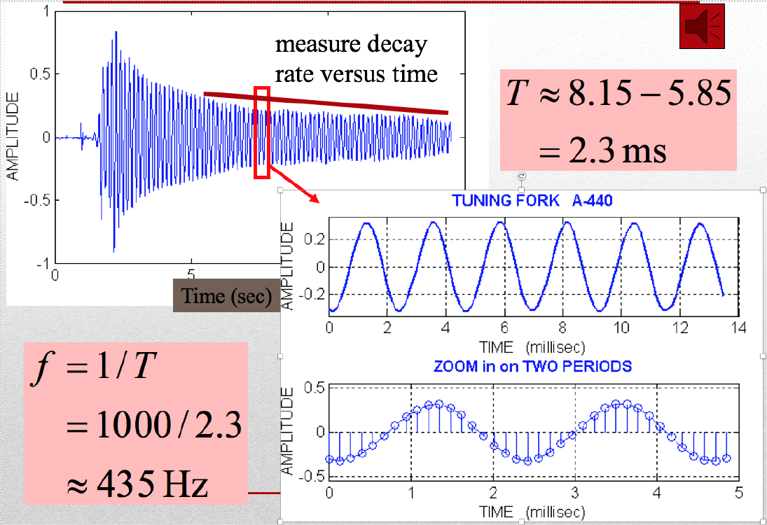
Figure \(\PageIndex{1}\): Example tuning fork recording. - Comment on the other signals present in the spectrum. Why don’t you see a nice clean delta function in the frequency plot?
-
Signal Source Frequency Estimate from Time Plot (Hz) Magnitude Decay Rate (V/s) Frequency Estimate from Frequency Plot (Hz) Tuning fork labeled 1024 Signal generator 440 Hz N/A
Report Checklist
Be sure the following are included in your report.
- All your MATLAB code in an appendix of the report (including your FFTPlot function)
- Section 4.3: Time and frequency plots of data measured from a tone generator app
- Section 4.3: Time and frequency plots of data measured from a tuning fork
- Section 4.3: Frequency measurements of the tone generator app’s signal from time and frequency plots (report in table)
- Section 4.3: Frequency measurements of the tuning fork from time and frequency plots (report in table)
- Section 4.3: Explanation of discrepancies between measured and expected frequencies
- Section 4.3: Plot and measurement of tuning fork amplitude decay (report estimate in table)
- Section 4.3: Comment on other signals in the spectrum