1.3: Impulse Response and Auralization

Learning Objectives

By the end of this lab, students will be able to:

1. Use a real-world impulse response to simulate different environments using discrete-time convolution
2. Describe FM modulated signals and chirp signals
3. Interpret a spectogram

Overview

“Auralization” is the process of using a computer to create or reproduce sound, often to achieve a desired sound effect. This is done by simulating characteristics of a room or other environment in order to produce sound that seems to have been recorded in that environment. Auralization is an increasingly popular technique for accurately simulating reverberation using acoustic impulse responses (IRs) from interesting buildings, spaces, and other sources. It is also used in video game and film production to create realistic sound effects.

Bring headphones to this lab!

Pre-Lab Reading

Auralization and Background

EchoThief (http://www.echothief.com) collects interesting IRs from “unusually clamorous places” for anyone to use. You can read about how these IRs are created here. A similar process is described in Section 3.1.1 This lab will use the computed impulse responses to approximate the sound of a signal in different environments.

Signal Acquisition

Ideally, we could obtain the acoustic impulse response of a space by producing an impulse signal and measuring the sound it produces in a given space. Unfortunately, impulse functions can only be approximated in the real world. One way to do this is to produce a short, tall (i.e., loud) pulse, but this requires a large amount of power (equal to the energy of the pulse divided by the pulse width). Requiring both more energy and a shorter pulse makes electrical power handling a limiting factor in such a system. The output stage of a transmitter can only handle so much power without destroying itself.

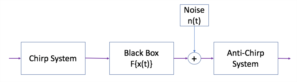
Chirp signals provide a way of breaking this limitation while still exciting a broad range of frequencies. (Knowing the impulse response is equivalent to knowing how the system responds to a sinusoid at any frequency.) A chirp signal is a sinusoid whose frequency changes from a starting frequency to an ending one. To generate a chirp, an impulse is passed through a chirp system. After the chirp echoes are received, the signal is passed through an antichirp system which converts the chirp echoes to an impulse response as shown in Figure 1 below. This phenomenon is called waveshaping. Often a logarithmically swept sine wave is used as a chirp signal.

Figure \(\PageIndex{1}\): An impulse response measurement system

Chirp Signals

Many interesting signals can be produced by changing the argument of a generalized sinusoid as different functions of time. This is called FM synthesis or Frequency Modulation¹ and is used to create instrument simulations, interesting sound effects, improve performance of radar systems, etc. A chirp signal is a sinusoid whose frequency sweeps from a starting frequency to an ending one. A “standard” sinusoid has \[\begin{aligned} x(t) &= A \cos{(\Psi(t))} & \Psi(t) = \omega t + \phi\end{aligned} \nonumber \] However, much more interesting signals can be created with different functions such as a quadratic, logarithmic, or sinusoid as shown below. \[\begin{aligned} \Psi(t) &= 2\pi \mu t^2 + 2 \pi f_0 t + \phi \\ \Psi(t) &= e^{a t} + 2 \pi f_0 t + \phi \\ \Psi(t) &= \cos{(2\pi f_1 t)} + 2 \pi f_0 t + \phi\end{aligned} \nonumber \]

The frequency spectra of these signals are hard to analyze; however, a decent approximation of signal behavior can be found by looking at the first derivative of the argument function. This is known as the instantaneous frequency, \(f_i\), of the signal. The instantaneous frequency of the linear, quadratic, and logarithmic chirp are: \[\begin{aligned} Linear: && f_i(t) = f_0 + \beta t && \beta = \frac{f_1-f_0}{t_1} & \\ Quadratic: && f_i(t) = f_0 + \beta t^2 && \beta = \frac{f_1-f_0}{t_1^2} & \\ Logarithmic: && f_i(t) = f_0 \beta^t && \beta = \left(\frac{f_1}{f_0}\right)^{1/t_1} &\end{aligned} \nonumber \]

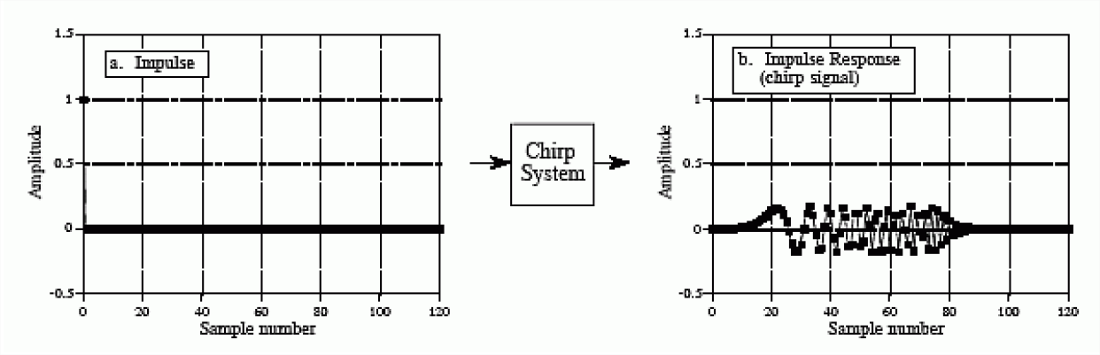
Figure \(\PageIndex{2}\) below shows the linear chirp system. For the problem of auralization, a logarithmically swept sinusoid is used.

Figure \(\PageIndex{2}\): Impulse response of a linear chirp signal (from Figure 11-10 of The Scientist and Engineer’s Guide to Signal Processing by Steven W. Smith, )

These signals can be generated using the Matlab command chirp.

y = chirp(t,f0,t1,f1,‘method’,phi)

The command generates samples of a swept-frequency cosine signal at the time instances defined in array t, where f_0 is the instantaneous frequency at time \(0\), and f_1 is the instantaneous frequency at time \(t_1\). f_0 and f_1 are both in hertz. If unspecified, \(f_0 = e^{-6}\) for logarithmic chirp and \(0\) for all other methods, \(t_1=1\), and \(f_1=100\).

Spectrograms

In addition to looking at signals in the time domain, it is often useful to look at the spectrum of a signal. A signal’s spectrum shows which frequencies are present in the signal. A constant frequency sinusoid spectrum consists of two impulse functions at \(\pm 2 \pi f_0\). For more complicated signals, there may be many spikes. For even more complicated signals such as music or frequency modulated signals, the spectrum changes with time. In these cases, the spectrogram of a signal is used instead of a spectrum. A spectrogram is found by estimating the spectrum over multiple short windows of time. The magnitude of the spectrum over these time “windows” is plotted as intensity or color on a two dimensional plot with time on one axis and frequency on the other.

In Matlab, the function spectrogram will be used to compute the spectrogram. The spectrogram function divides a signal into segments. Longer segments provide better frequency resolution; shorter segments provide better time resolution. For more information, see http://www.mathworks.com/help/signal/examples/practical-introduction-to-time-frequency-analysis.html. There are theoretical limits on how well short pieces of the signal can represent the frequency content in a signal. Generally, longer time windows give better frequency resolution. The spectrogram function can be called as follows: spectrogram(xx, 1024, 512, [], Fs). The first argument, xx, is the time signal, 1024 is the number of samples in the time window, 512 is the number of samples of overlap between the time windows, and Fs is the sampling frequency. NOTE: the spectrogram function requires the Matlab signal processing toolbox.

In order to see what the spectrogram function does, run the following code.

N = 1024;
n = (0:N-1);
w0 = 2*pi/5;
x = sin(w0*n)+10*sin(2*w0*n);
spectrogram(x,128,64,[],100);

To see the spectrogram of a chirp, replace x = sin(w0*n)+10*sin(2*w0*n); with a chirp signal.

Lab Exercises

Using a Computed Impulse Response and Convolution

Implement sound effects on a provided sound clip and impulse responses of your choice.

1. Go to EchoThief and select an interesting location. Download the impulse response associated with the place you chose. The file you downloaded should be a .wav file.
2. Examine your impulse response. To do this, you will first need to load it into MATLAB using [v, Fs] = audioread(file.wav). What is the sampling rate of this impulse response? How many samples long is your IR? How long in seconds is your IR? Plot your IR as a function of time, with the time in seconds. Comment on the plot in your report. Is this a mono or stereo recording? You can listen to your IR by typing soundsc(v, Fs) in MATLAB.
3. Download one of the two voice files from Canvas (female voice: spfe49_1.wav or male voice: spme50_1.wav). Load this audio file into MATLAB. What is the sampling rate of this file? Is this a mono or stereo recording? How many samples are in the signal? Listen to the audio. What is the voice talking about?
4. Now for the fun part! We want to make it sound like the voice is coming from the location corresponding to your IR. We can do this by convolving the speach signal with the impulse response. Suppose your voice signal is \(v[n]\) and the IR is \(h[n]\). The convolution \(y[n] = v[n]*h[n]\) will produce a speach signal that sounds like it was recorded at the location you picked. It MATLAB, you can type y = conv(v,h) to convolve the signals.
   1. NOTE 1: make sure your voice signal and IR are recorded at the same sampling rate, otherwise you will need to use resample on one of them.
   2. NOTE 2: if your voice signal or IR (or both) were recorded in stereo, you will have to pick one of the two channels to use before calling conv. You can select the first column of a matrix \(\mathbf{h}\) by typing h1 = h(:,1).
5. You can play back your new voice by typing soundsc(y,Fs).² Describe what you hear in your report.
6. Feel free to experiment with IRs from different locations and different sound files, but leave enough time to finish Section 4.2.

Investigating Frequency Modulated (FM) Signals

A chirp signal is also known as a swept frequency cosine. The frequency of the cosine changes in time. The frequency can change in many different ways as seen in Figure Figure \(\PageIndex{3}\) for linear and quadratic sweeps. We will focus on a linear sweep where the instantaneous frequency is linear as shown in Figure \(\PageIndex{3(left)}\). Figure Figure \(\PageIndex{3(right)}\) shows the case where the instantaneous frequency is a quadratic.

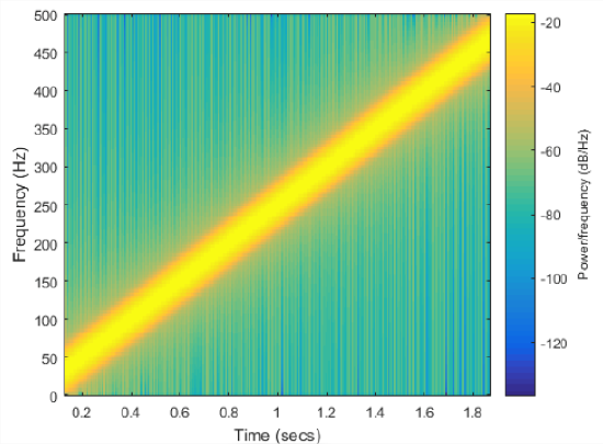
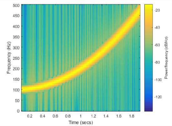
Figure \(\PageIndex{3}\): (left) Linear chirp and (right) quadratic chirp

1. Use the Matlab chirp command to generate a signal. Find the spectrogram using a window length of 2048 using the command:

   spectrogram(x,2048,1024,[],Fs,`yaxis'); 

   Include this plot in your lab report and comment on the shape of the chirp.

2. What is the frequency value at \(t=1.0\) sec for the chirps in Figure \(\PageIndex{3}\) ?
3. As a test case, generate a chirp sound whose frequency starts at 400 Hz and ends at 4000 Hz with a duration of seven seconds and a sampling rate of 44.1 kHz. Listen to the sound that the chirp makes using the soundsc command in Matlab and include a listing of the commands that you used to generate the chirp signal and spectrogram.
4. Synthesize a “chirp” signal with the following parameters: time duration of five seconds with a sampling frequency of 11,025 Hz, starting frequency of 5000 Hz, and ending frequency of 20 Hz. Listen to the signal; what does it sound like (e.g., is the frequency movement linear)? Does it chirp down or up? Create a spectrogram of the signal to verify that you have the correct instantaneous frequency.
5. Synthesize a “chirp” signal with the following parameters: time duration of ten seconds with a sampling frequency of 11,025 Hz, starting frequency of 20 Hz, and the frequency at time \(t=1\) sec should be 1200 Hz. Listen to the signal; what does it sound like (e.g., is the frequency movement linear)? Does it chirp down or up? Create a spectrogram of the signal to verify that you have the correct instantaneous frequency. Speculate on what is happening with the signal.

Report Checklist

Be sure the following are included in your report.

Section 4.1

1. Characteristics of the impulse response you chose (length in sec, length in samples, sampling rate)
2. Plot of your IR and comments about it
3. Description of the voice you chose (sampling rate, mono/stero, number of samples, etc.)
4. Description of your sound effect

Section 4.2

1. Plot of your chirp with comments
2. Frequency values from Figure \(\PageIndex{3}\)
3. Spectrogram of seven second chirp with code in the appendix
4. Description of five second chirp with spectrogram
5. Description of ten second chirp with spectrogram

9 “EchoThief Impulse Response Library,” EchoThief, SuperHoax,
http://www.echothief.com/

Steven W. Smith. The Scientist and Engineer’s Guide to Digital Signal Processing, California Technical Publishing, San Diego, CA, 1997.

Michael Vorländer. Auralization : Fundamentals of Acoustics, Modelling, Simulation, Algorithms and Acoustic Virtual Reality, Springer, Berlin, Germany, 2008.

---

1. In FM radio, the argument of the sinusoid contains the audio signal.↩
2. Be sure to use soundsc. The sound function expects to get data ranging from -1.0 to 1.0 (see the help documentation), so if your audio signal exceeds 1.0 in magnitude, you will here additional distortion not caused by your IR.↩