
1.4: Frequency Response - Notch and Bandpass Filters
- Page ID
- 96176
By the end of this lab, students will be able to:
- Plot the frequency response of an FIR filter
- Implement and apply an FIR filter in MATLAB
- Design an FIR filter for nulling frequency components
- Design an FIR filter for isolating specific frequencies
Overview
The goal of this lab is to study the response of finitie impulse response (FIR) filters to inputs such as complex exponentials and sinusoids. In the experiments, you will use MATLAB’s conv function to implement filters in the time domain and freqz to obtain each filter’s frequency response. As a result, you should learn how to characterize a filter by knowing how it reacts to different frequency components in the input. This lab also introduces two practical filters: bandpass filters and nulling filters. Bandpass filters can be used to detect and extract information from sinusoidal signals, e.g., tones in a touch-tone telephone dialer. Nulling filters can be used to remove sinusoidal interference, e.g., jamming signals in a radar or 60 Hz power signals from lights.
Pre-Lab Reading
Frequency Response of FIR Filters
The output or response of a filter for a complex sinusoidal input, \(e^{j \Omega}\), depends on the frequency, \(\Omega\). Often a filter is described solely by how it affects different input frequencies–this is called the frequency response. For example, the frequency response of the two-point averaging filter \[\begin{aligned} y[n] &= \frac{1}{2}x[n] + \frac{1}{2}x[n-1]\end{aligned} \nonumber \] can be found by using a general complex exponential as an input and observing the output or response. \[\begin{aligned} x[n] &= A e^{j (\Omega n + \phi)} \nonumber \\ y[n] &= \frac{1}{2} A e^{j ( \Omega n + \phi)} + \frac{1}{2} A e^{j (\Omega (n-1) + \phi)} \nonumber \\ &= A e^{j (\Omega n + \phi)} \frac{1}{2}\left( 1+e^{-j \Omega} \right) \nonumber \\ &= A e^{j (\Omega n + \phi)} H\left( e^{j \Omega} \right) \label{eq:freqresp}\end{aligned} \] In [eq:freqresp] there are two terms, the original input and a term that is a function of \(\Omega\). This second term is the frequency response, and it is commonly denoted by \(H(e^{j\Omega})\), which in this case is \[\begin{aligned} H(e^{j\Omega}) &= \frac{1}{2}\left( 1+e^{-j \Omega} \right)\end{aligned} \nonumber \] Once the frequency response, \(H(e^{j\Omega})\), has been determined, the effect of the filter on any complex exponential may be determined by evaluating \(H(e^{j\Omega})\) at the corresponding frequency. The output signal, \(y[n]\), will be the original input complex exponential signal times a complex number. The phase of this number imparts a phase shift and the magnitude describes the gain applied to the complex exponential. The frequency response of a general finite impulse response (FIR) linear, time-invariant system is \[\begin{aligned} H(e^{j\Omega}) &= \sum_{k=0}^{M} b_k e^{-j \Omega k} \label{eq:frFIR}\end{aligned} \] In the example above, \(M=1\) and \(b_0 = b_1 = \frac{1}{2}\).
MATLAB Function for Frequency Response
MATLAB has a built-in function called freqz for computing the frequency response of a discrete-time LTI system. The following MATLAB statements show how to use freqz1 to compute and plot both the magnitude (absolute value) and the phase of the frequency response of a two-point averaging system as a function of \(\Omega\) in the range \(-\pi \leq \Omega \leq \pi\):
bb = [0.5, 0.5]; \% Filter Coefficients
ww = -pi:(pi/100):pi; \% omega
HH = freqz(bb, 1, ww);
subplot(2,1,1);
plot(ww, abs(HH));axis([-pi,pi,0,1]);
subplot(2,1,2);
plot(ww, angle(HH));axis([-pi,pi,-2,2]);
xlabel(`Normalized Radian Frequency')
For FIR filters, the second argument of freqz must always be equal to 1. The frequency vector ww should cover an interval of length \(2\pi\) for \(\Omega\), and its spacing must be fine enough to give a smooth curve for \(H(e^{j \Omega})\). Note: we will always use capital HH for the frequency response in this lab.
Periodicity of the Frequency Response
The frequency responses of discrete-time filters are always periodic with period equal to \(2 \pi\). Explain why this is the case by stating a definition of the frequency response and then considering two input sinusoids whose frequencies are \(\Omega\) and \(\Omega + 2 \pi\): \[\begin{aligned} x_1[n] &= e^{j \Omega n} \\ x_2[n] &= e^{j \Omega n + 2 \pi n}\end{aligned} \nonumber \] Notice that \(x_2[n] = x_1[n]\), so the output will be the same for both inputs. Include your answer in your lab report.
The implication of periodicity is that a plot of \(H(e^{j \Omega})\) only needs to extend over the interval \(-\pi \leq n \leq \pi\) or any other interval of length \(2\pi\).
Lab Exercises
Frequency Response of the Four-Point Averager
Filters that average input samples over a certain interval are called “running average” filters or “averagers,” and they have the following form (for an \(L\)-point averager): \[\begin{aligned} y[n] &= \frac{1}{L} \sum_{k=0}^{L-1} x[n-k]\end{aligned} \nonumber \] In other words, the impulse response of an \(L\)-point averager is: \[\begin{aligned} h[n] &= \begin{cases} \frac{1}{L} & 0 \leq n \leq L-1 \\ 0 & \textrm{otherwise} \end{cases}\end{aligned} \nonumber \]
- Use Euler’s formula, [eq:frFIR], and complex number manipulations to show that the frequency response for the 4-point running average operator is given by: \[\begin{aligned} H\left( e^{j \Omega} \right) &= \frac{\cos{(0.5 \Omega)} + \cos{(1.5 \Omega)}}{2} e^{-j 1.5 \Omega} \label{eq:4pnt}\end{aligned} \]
- Implement [eq:4pnt] directly in MATLAB and plot the frequency response. Use a vector that includes 400 samples between \(-\pi\) and \(\pi\) for \(\Omega\). Since the frequency response is a complex-valued quantity, use
absandangleto extract the magnitude and phase of the frequency response for plotting. Plotting the real and imaginary parts of \(H(e^{j\Omega})\) is not very informative. - Use
freqzin MATLAB to compute \(H(e^{j\Omega})\) numerically (from the filter coefficients) and plot its magnitude and phase versus \(\Omega\). Include the appropriate MATLAB code to plot both the magnitude and phase of \(H(e^{j\Omega})\) in your lab report’s appendix. Follow the example in Section 3.2. The filter coefficient vector for the 4-point averager is defined via:bb = 1/4*ones(1,4);Note: the function
freqz(bb,1,ww)evaluates the frequency response for all frequencies in the vectorww. It uses the summation in [eq:frFIR], not the formula in [eq:4pnt]. The filter coefficients are defined in the assignment to vectorbb. How do your results compare with part (b)?
The MATLAB find Function
Often signal processing functions are performed in order to extract information that can be used to make a decision. The decision process inevitably requires logical tests, which might be done with if-then constructs in MATLAB. However, MATLAB permits vectorization of such tests, and the find function is one way to do lots of tests at once. In the following example, find extracts all the numbers that “round” to 3:
xx = 1.4:0.33:5, jkl = find(round(xx)==3), xx(jkl)The argument of the find function can be any logical expression. Notice that find returns a list of indices where the logical condition is true. See help on relop for information.
Now, suppose that you have a frequency response:
ww = -pi:(pi/500):pi; HH = freqz( 1/4*ones(1,4), 1, ww );Use the find command to determine the indices where HH is zero, and then use those indices to display the list of frequencies where HH is zero. Since there might be round-off error in calculating HH, the logical test should probably be a test for those indices where the magnitude (absolute value in MATLAB) of HH is less than some rather small number, e.g., \(1 \times 10^{-6}\). Compare your answer to the frequency response that you plotted for the four-point averager in Section 4.1.
Nulling Filters for Rejection
Nulling filters are filters that completely eliminate some frequency component. If the frequency is \(\Omega = 0\) or \(\Omega = \pi\), then a two-point FIR filter will do the nulling. The simplest possible general nulling filter can have as few as three coefficients. If \(\Omega\) is the desired nulling frequency, then the following length-3 FIR filter will have a zero in its frequency response at \(\Omega = \Omega_n\): \[\begin{aligned} y[n] &= x[n] - 2 \cos{(\Omega)} x[n-1] + x[n-2]\end{aligned} \nonumber \] For example, a filter designed to completely eliminate signals of the form \(A e^{j 0.5 \pi n}\) would have the following coefficients because we would pick the desired nulling frequency to be \(\Omega_n = 0.5 \pi\). \[\begin{aligned} b_0 = 1, && b_1 = -2 \cos{(0.5 \pi )} = 0, && b_2 = 1\end{aligned} \nonumber \]
- Design a filtering system that consists of the cascade of two FIR nulling filters that will eliminate the following input frequencies: \(\Omega = 0.44 \pi\), and \(\Omega = 0.7 \pi\). For this part, derive the filter coefficients of both nulling filters.
- Generate an input signal \(x[n]\) that is the sum of three sinusoids: \[\begin{aligned} x[n] = 5 \cos{(0.3 \pi n)} + 22 \cos{\left(0.44 \pi n - \frac{\pi}{3} \right)} + 22 \cos{\left(0.7 \pi n - \frac{\pi}{4}\right)}\end{aligned} \nonumber \] Make the input signal 150 samples long over the range \(0\leq n \leq 149\).
- Use
convto filter the sum of three sinusoids signal \(x[n]\) through the filters designed in part (a). Include the MATLAB code that you wrote to implement the cascade of two FIR filters in the appendix. - Make a plot of the output signal and show the first 40 points. Determine (by hand) the exact mathematical formula (magnitude, phase, and frequency) for the output signal for \(n \geq 5\). (Hint: recall that an LTI system alters the magnitude and phase of sinusoidal inputs.)
Simple Bandpass Filter Design
The \(L\)-point averaging filter is a lowpass filter. Its passband width is controlled by \(L\), being inversely proportional to \(L\). It is also possible to create a filter whose passband is centered around some frequency other than zero. One simple way to do this is to define the impulse response of an \(L\)-point FIR as: \[\begin{aligned} h[n] = \frac{2}{L} \cos{(\Omega_c n)}, && 0 \leq n < L\end{aligned} \nonumber \] where \(L\) is the filter length and \(\Omega_c\) is the center frequency that defines the frequency location of the passband. For example, we would pick \(\Omega_c = 0.44 \pi\) if we want the peak of the filter’s passband to be centered at \(0.44\pi\). The bandwidth of the bandpass filter (BPF) is controlled by \(L\); the larger the value of \(L\), the narrower the bandwidth.
- Generate a bandpass filter that will pass a frequency component at \(\Omega = 0.44\pi\). Make the filter length (\(L\)) equal to 10. Since we are going to be filtering the signal defined below, measure the gain of the filter at the three frequencies of interest: \(\Omega = 0.3\pi\), \(\Omega = 0.44\pi\) and \(\Omega = 0.7\pi\). \[\begin{aligned} x[n] &= 5 \cos{(0.3 \pi n)} + 22 \cos{\left(0.44 \pi n - \frac{\pi}{3} \right)} + 22 \cos{\left(0.7 \pi n - \frac{\pi}{4}\right)} \label{eq:3tone}\end{aligned} \]
- The passband of the BPF is defined by the region of the frequency response where \(|H(e^{j \Omega})|\) is close to its maximum value. If we define the maximum to be \(H_{max}\), then the passband width is defined as the length of the frequency region where the ratio \(|H(e^{j\Omega})|/H_{max}\) is greater than \(1/\sqrt{2} = 0.707\). The stopband of the BPF filter is defined by the region of the frequency response where \(|H(e^{j\Omega})|\) is close to zero. In this case, we will define the stopband as the region where \(|H(e^{j\Omega})|\) is less than 25% of the maximum.
Figure 1 shows how to define the passband and stopband. Note: you can use MATLAB’s
findfunction to locate those frequencies where the magnitude satisfies \(|H(e^{j \Omega})| \geq 0.707 H_{max}\).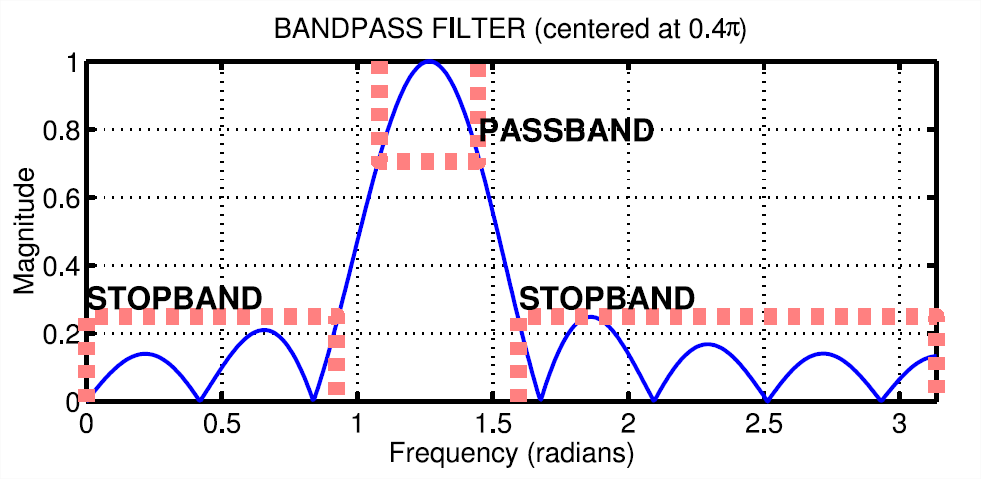
Figure \(\PageIndex{1}\): Passband and Stopband for a typical FIR bandpass filter. In this case, the maximum value is 1, the passband is the region where the frequency response is greater than \(1/\sqrt{2} = 0.707\) times the maximum value, and the stopband is defined as the region where the frequency response is less than 25% of the maximum. Make a plot of the frequency response for the \(L = 10\) bandpass filter from part (a), and determine the passband width (at the 0.707 level). Repeat the plot for \(L = 20\) and \(L = 40\) so you can explain how the width of the passband is related to filter length \(L\), i.e., what happens when \(L\) is doubled or halved.
- Comment on the selectivity of the \(L = 10\) bandpass filter. In other words, which frequencies are “passed by the filter”? Use the frequency response to explain how the filter can pass one component at \(\Omega = 0.44 \pi\), while reducing or rejecting the others at \(\Omega = 0.3 \pi\) and \(\Omega = 0.7 \pi\).
- Generate a bandpass filter that will pass the frequency component at \(\Omega = 0.44 \pi\), but now make the filter length (\(L\)) long enough so that it will also greatly reduce frequency components at (or near) \(\Omega = 0.3 \pi\) and \(\Omega = 0.7 \pi\). Determine the smallest value of \(L\) so that
- Any frequency component satisfying \(|\Omega| \leq 0.3 \pi\) will be reduced by a factor of 10 or more2.
- Any frequency component satisfying \(0.7 \pi \leq |\Omega| \leq \pi\) will be reduced by a factor of 10 or more.
This can be done by making the passband width very small.
- Use the filter from the previous part to filter the “sum of three sinusoids” signal in \ref{eq:3tone}. Make a plot of 100 points of the input and output signals, and explain how the filter has reduced or removed two of the three sinusoidal components.
- Make a plot of the frequency response (magnitude only) for the filter from part (d), and explain how \(H(e^{j\Omega})\) can be used to determine the relative size of each sinusoidal component in the output signal. In other words, connect a mathematical description of the output signal to the values that can be obtained from the frequency response plot.
Report Checklist
Be sure the following are included in your report.
- Section 3.3: explanation of periodicity of frequency response
- Section 4.1: derivation of [eq:4pnt]
- Section 4.1: (labeled) plots of magnitude and phase of \(H(e^{j \Omega})\)
- Section 4.1: plots of \(H(e^{j \Omega})\) using
freqz(code in appendix) - Section 4.2: list of frequencies where
HHis 0 (and compare to above) - Section 4.3: coefficients of two nulling filters
- Section 4.3: MATLAB code for filtering signal (appendix)
- Section 4.3: plot of nulled output and formula for output signal
- Section 4.4: coefficients of bandpass filter; gain at three frequencies
- Section 4.4: plots of frequency response for \(L = 10\), \(20\), and \(40\) with a description of the passband widths
- Section 4.4: comments on selectivity of the \(L=10\) BPF
- Section 4.4: the smallest \(L\) that satisfies the criteria
- Section 4.4: plot of input and output; explanation of effect on three sinusoid signal
- Section 4.4: plot of frequency response; explanation of size of each sinusoidal component in output
- If the output of the
freqzfunction is not assigned, then plots are generated automatically; however, the magnitude is given in decibels which is a logarithmic scale. For linear magnitude plots a separate call toplotis necessary.↩ - For example, the input amplitude of the \(0.7\pi\) component is 22, so its output amplitude must be less than 2.2↩