1.6: Introduction to Digital Images

Learning Objectives

By the end of this lab, students will be able to:

1. Describe digital image types, including monochrome and color.
2. Display images in MATLAB.
3. Perform basic pixel manipulation including clearing, copying, inverting, and thresholding.
4. Perform grsyscale brightening and contrast-stretching.

Overview

In this lab we introduce digital images as a new higher dimensional signal type. Digital images are written as two-dimensional matrices of numbers that can be manipulated to enhance contrast, invert images, and highlight objects.

Pre-Lab Reading

Monochrome Images

An image can be represented as a function \(J(x, y)\) of two continuous variables representing the horizontal (\(x\)) and vertical (\(y\)) coordinates of a point in space. The variables \(x\) and \(y\) represent spatial dimensions. Thus, their units would be inches or some other unit of length. Moving images (such as video) add a time variable to the two spatial variables. Digital images sample the signal \(J(x,y)\) at uniform intervals: \[\begin{aligned} J[m,n] &= J(mT_1, nT_2) &1 \leq m \leq M \textrm{ and } 1\leq n \leq N\end{aligned} \nonumber \] where \(T_1\) and \(T_2\) are the sample spacings in the horizontal and vertical directions. In MATLAB, we can represent an image as a matrix which consists of M rows and N columns. The matrix entry at \((m, n)\) is the sample value \(J[m, n]\)—called a pixel (short for picture element).

Monochrome images are displayed using black and white and shades of gray, so they are called grayscale images. In this lab, we will consider only sampled grayscale still images. A sampled grayscale still image would be represented as a two-dimensional array of numbers. An important property of light images such as photographs and TV pictures is that their values are always non-negative and finite in magnitude; i.e., \[\begin{aligned} 0 \leq J[m,n] \leq J_{max} < \infty\end{aligned} \nonumber \] This is because light images are formed by measuring the intensity of reflected or emitted light which must always be a positive, finite quantity. When stored in a computer or displayed on a monitor, the values of \(J[m, n]\) have to be scaled relative to a maximum value \(J_{max}\) . Usually, an eight-bit integer representation is used. With 8-bit integers, the maximum value (in the computer) would be \(J_{max} = 2^8 -1 = 255\), and there would be \(2^8 = 256\) different gray levels for the display, from 0 to 255. Images in this format have type uint8 (unsigned 8-bit integer) in MATLAB. However, in image recognition applications, binary images (\(J_{max}=1\)) are often used to separate parts of the image that are of interest from areas that are not. A simple example is the application of zip code recognition on letters. The algorithm would first search for the zip code, then filter out the rest of the image.

Displaying and Exporting Images in MATLAB

Most of the lab exercises in this class will require you to produce one or more output images. These will need to be incorporated into your report. Since many exercises will use MATLAB, we will describe here some basic I/O and display commands in the MATLAB environment.

• Reading Images: You can read an image file, img.tif or image.jpg, into the MATLAB workspace using the command:

  IMG=imread(’pout.tif’);

  This will produce an image matrix IMG of data type uint8.

• Displaying Images: You can display the image array IMG with the following commands.

  colormap(gray(256));  % only needed for grayscale image
  imshow(IMG)
  truesize; 

  If IMG is a grayscale image, the colormap function is needed to tell MATLAB which color to display for each possible pixel value. The truesize command, which is included in the image processing toolbox, maps each image pixel to a single display pixel to avoid any interpolation on the display. This will be important in future labs.

• Writing Images: When producing a lab report document, you should strive to present the best representation of your output images. Therefore, it is best to export your images to a lossless file format, such as TIFF or BMP, which can then be imported into your lab report document. You can write the image array X to a file using the imwrite function:

  imwrite(x,’img_out.tif’)

  Note that if X is of type uint8, the imwrite function assumes a dynamic range of \([0,255]\), and will clip any values outside that range. If X is of type double, then imwrite assumes a dynamic range of \([0,1]\), and will linearly scale to the range \([0,255]\), clipping values outside that range, before writing out the image to a file. To convert the image to type uint8 before writing, you can use

  imwrite(uint8(x),’img_out.tif’)

  If your image is in color, such as RGB (Red-Green-Blue), then you will need to convert it to grayscale using the rgb2gray command in MATLAB:

  RGB = imread(`peppers.png'); imshow(RGB)
  I = rgb2gray(RGB);
  figure; imshow(I)

Prelab Questions

Open Matlab and run the following command:

moon = imread(`moon.tif');

1. What is the size of the image example? NxM pixels
2. What is the variable type?
3. Write out one line of Matlab code for seeing the intensity value of any given pixel in the image.

Image Manipulation

The goal of image manipulation is to improve the image in ways that increase the performance of a system for human viewing or computer vision applications.

Histogram Computation

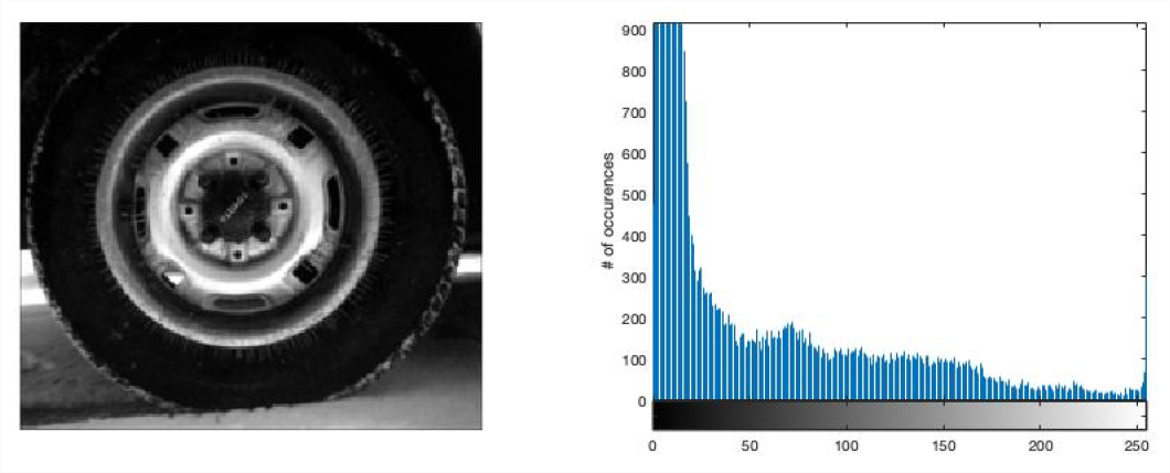
Image histograms are a simple but very useful method to analyze images and to enhance the quality of the image (at least for a human observer) by performing point transformations. In grayscale images, the histogram looks at the distribution of the intensity values of the image. For each range of grayscale values, the number of pixels in that range are counted. To see the distribution of intensities in the image, create a histogram by calling the imhist function. Generally, a good contrast image will have values spread out across the range of the intensity values from \(0\) to \(N\). Figure \(\PageIndex{1}\) shows the MATLAB image tire.tif and its histogram. Note that most of the pixels have low values that are in the range of 0-25 in intensity.

Figure \(\PageIndex{1}\): Image of a tire with a histogram of intensity values. Most of the pixels have low intensities.

Contrast Stretching and Intensity Level Slicing

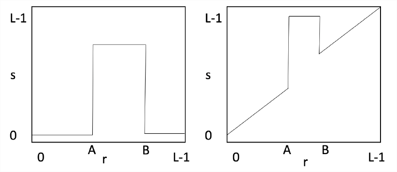
Low contrast images result from poor illumination or lack of response from the imaging sensor. The idea behind contrast stretching is to increase the dynamic range of the gray levels in the image being processed. This is implemented by a mapping function, \(s = T(r)\). Figure 2 shows a typical transformation for contrast stretching. The locations of points \((r1, s1)\) and \((r2,s2)\) control the shape of the contrast function. If \(r1=r2\) and \(s1=s2\), then the transformation is a linear function. If \(r1=r2\), \(s1=0\), and \(s2=L-1\), then the transformation is a thresholding function. Intermediate values produce different types of spread. The mapping is a piecewise linear interpolation.

Figure \(\PageIndex{2}\): Example contrast mapping \(s = T(r)\). The function \(T\) is applied to each pixel.

A related transformation is Intensity Level Slicing which can highlight or delete a specific range of gray levels. Applications include enhancing features such as water in satellite images or the tire in the image above. There are two main approaches for this: display a high value for all of the pixels in a desired range and zero out the others or brighten the pixels in the range and leave the other pixels the same. Levels can be deleted using a similar approach. Examples are shown in Figure \(\PageIndex{3}\).

Figure \(\PageIndex{3}\): Example mapping functions for Intensity Level Slicing. The mapping on the left zeros out all pixels that have intensities below \(A\) (\(r<A\)) and above \(B\) (\(r>B\)). The mapping on the right brightens pixels with intensities between \(A\) and \(B\) (\(A\leq r \leq B\)).

Histogram Equalization

Figure \(\PageIndex{3}\): Tire image after histogram equalization with a histogram of its intensities.

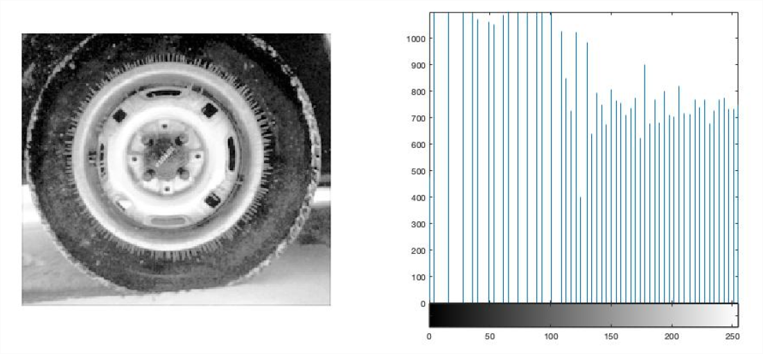
The histogram equalization operation tries to change the pixel distribution so that it is as close as possible to a uniform distribution. This means that all gray levels from \(0\) to \(2^{B}-1\) (where \(B\) is the number of bits) are approximately equally likely. The effect is to widen the effective dynamic range of the image intensity. The results for this operation are shown in Figure 4 for the tire.tif image. Compare this to the original image in Figure 1. Note that the histogram extends across most gray values with approximately equal numbers of occurrences. MATLAB code for this operation is (X is the original image):

Xeq = histeq(X);
figure; subplot(121); imshow(Xeq)
subplot(122); imhist(Xeq)

Lab Exercises

1. Load the image “pout.tif” into MATLAB and compute its histogram. Include the histogram and image in your lab report.
   1. What is the range of the pixel intensity values in the original image?
   2. Give two methods for increasing the range of the image intensity from Section 4 above. Describe and implement the methods and show the results of the operations in your lab report. Compare the results in both cases, does one method work better than the other?
2. Load the built-in MATLAB image “coloredChips.png.” You will need to convert the image to grayscale. Use the methods described in Section 4 to isolate the round chips in the image by filtering the image intensity. The goal is to pre-process the image to remove the background so that a machine vision system can easily count the chips on the table. In your lab report, describe what steps you took to analyze the image and subtract the background. Include your MATLAB script and the stages of your processing pipeline. Display the image after each processing step.

Report Checklist

Be sure the following are included in your report.

1. Section 3.3: answer the three pre-lab questions
2. Section 5: answer the questions and complete the exercises in 1(a) and 1(b)
3. Section 5: complete and describe your approach to isolating the chips in 2

Reference

9 R.C. Gonzalez and R.E. Woods Digital Image Processing, Addison Wesley, 1993

“MATLAB Image Processing Toolbox Documentation”,’ The Mathworks,
https://www.mathworks.com/help/images/index.html?s_tid=CRUX_lftnav

Jackson,Jeff Notes from ECE 482, University of Alabama,
jjackson.eng.ua.edu/courses/ece482/lectures/LECT01-2.pdf
jjackson.eng.ua.edu/courses/ece482/lectures/LECT05-2.pdf