
1.7: Filtering Digital Images
- Page ID
- 96180
By the end of this lab, students will be able to:
- Describe spatial frequency in 2D digital images.
- Design and implement linear, spatially invariant (LSI) filters using two-dimenional convolutional windows.
- Use the properties of LSI filters to implement the Canny Edge Detection Protocol for images.
Overview
In this lab, we introduce linear sliding window filtering of images. The filters work in two dimensions to enhance the image in ways such as averaging out noise or emphasizing edges.
Pre-Lab Reading and Exercises
Image Filtering and Spatial Frequency
Image analysis deals with techniques for extracting information from images. The first step is generally to segment an image. Segmentation divides an image into its constituent parts or objects. For example, in a military air-to-ground target acquisition application one may want to identify tanks on a road. The first step is to segment the road from the rest of the image and then to segment objects on the road for possible identification. Segmentation algorithms are usually based on one of two properties of gray-level values: discontinuity and similarity. For discontinuity, the approach is to partition an image based on abrupt changes in gray level. Objects of interest are isolated points, lines, and edges.
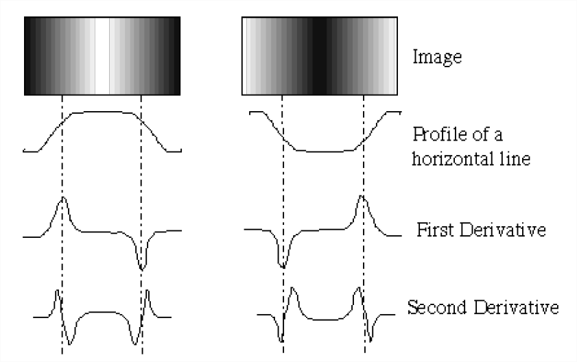
An edge is the boundary between two regions with relatively distinct gray-level properties. The idea underlying most edge-detection techniques is the computation of a relative derivative operator. Figure \(\PageIndex{1}\) illustrates this concept. The picture on the left shows an image of a light stripe on a dark background, the gray-level profile of a horizontal scan line, and the first and second derivatives of the profile. The first derivative is positive when the image changes from dark to light and zero where the image is constant. The second derivative is positive for the part of the transition associated with the dark side of the edge and negative for the transition associated with the light side of the edge. Thus, the magnitude of the first derivative can be used to detect the presence of an edge in the image and the sign of the second derivative can be used to detect whether a pixel lies on the light or dark side of the edge.
Sliding Window Filters
One way of filtering is to first filter the rows with a one-dimensional filter and then filter the columns with a one-dimensional filter. Alternatively, two dimensional filters can be applied to the neighborhood of each pixel to filter a signal. Filtering can help remove noise from an image by averaging out the effects of random noise fluctuations. High pass filters help detect edges and sudden spatial changes in an image.
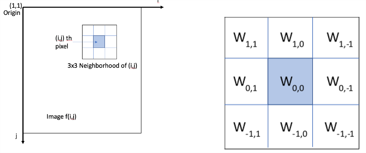
The operations take place in the spatial domain and operate directly on pixel values. The general form for operations is: \(y(i, j) = T[x (i, j)]\) where \(x(i,j)\) is the input image, \(y(i,j)\) is the filtered output image, \(T\) is an operator on \(x\) defined over a neighborhood of point \((i,j)\). The operator, \(T\), defines the size of the neighborhood around each pixel. The neighborhood is usually rectangular, centered on \((i,j)\) and is much smaller than the image. This neighborhood is moved around to each pixel, hence the name sliding window or spatial mask. Use of spatial masks for filtering is called spatial filtering and the masks can be linear or nonlinear. As a note, the linear filter is equivalent to a two-dimensional convolution of the image with the filter.
A three by three linear filter can be written in matrix form as: \[\begin{bmatrix} w_{1,1} & w_{1,0} & w_{1,-1} \\ w_{0,1} & w_{0,0} & w_{0,-1} \\ w_{-1,1} & w_{-1,0} & w_{-1,-1} \end{bmatrix} \nonumber \] The output of applying a three by three mask to image \(x\) is given by the two-dimensional convolution: \[\begin{aligned} y(i,j) &= \sum_{k=-1}^{1} \sum_{l=-1}^{1} w_{k,l} x(i-k,j-l) \\ &= w_{1,1} x(i-1,j-1) + w_{1,0} x(i-1,j) + w_{1,-1} x(i-1,j+1) \\ & \quad + w_{0,1} x(i,j-1) + w_{0,0} x(i,j) + w_{0,-1} x(i,j+1) \\ & \quad + w_{-1,1} x(i+1,j-1) + w_{-1,0} x(i+1,j) + w_{-1,-1} x(i+1,j+1) \\\end{aligned} \nonumber \]
This masking process continues until all pixels in the image are covered. The standard practice is to create a new image with the new values. For pixels near the boundary of the image, the output may be computed using partial neighborhoods or by padding the input appropriately by adding in repeated edge rows/columns or by a frame of black or white pixels.
These types of spatial filters are linear and spatially invariant (LSI). They can also be interpreted in the frequency domain. Lowpass filters attenuate (or eliminate) high frequency components characterized by edges and sharp details in an image with the net effect of blurring the image. Highpass filters attenuate (or eliminate) low frequency components such as slowly varying characteristics. The overall effect is a sharpening of edges. Bandpass filters attenuate (or eliminate) a given frequency range of frequencies. This is primarily used for image restoration.
Technical Notes for Implementing Filter Masks
In this lab, the MATLAB routine imfilter will be used: Y = imfilter(X,h); where \(X\) is the image to be filtered, \(h\) is the filter in matrix form, and \(Y\) is the filtered image. A simple example for a three by three averaging filter is given below:
>>X=imread(‘moon.tif’);
>>h = ones(3)/9;% or [1,1,1;1 1 1;1 1 1]/9;
>>Y = imfilter(X,h);
There are two things to keep in mind with imfilter. First, it returns an image in the same format as the input. This means that if, for a uint8 image, the function gets a non-integer value, it rounds it to the closest integer. Second, it clips pixel values outside of the range [0, 255] to 0 or 255. These are non-linear operations which effect whether the LSI operations can be done in any order. For pixels near the boundary of the image, the output may be computed using partial neighborhoods or by padding the input appropriately by adding in repeated edge rows/columns or by a frame of black or white pixels. The default in imfilter is to assume a black border. Details can be found by reading about padding options on the help page.
Pre-Lab Questions
- Which part of the image in Figure \(\PageIndex{3}\) has the lowest spatial frequency: specify top, bottom, left, right, middle, or a corner.
Figure \(\PageIndex{3}\): Image for question 1. - Compute the spatial period of the image below in terms of pixels/cycle. Give a numerical answer.
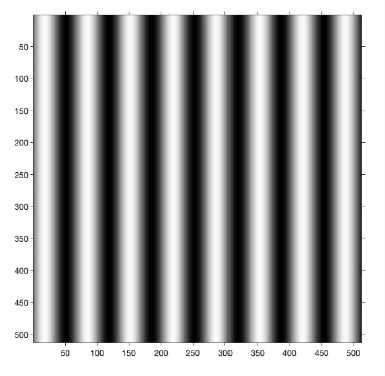
Figure \(\PageIndex{3}\): Image for question 2. - Given the 2D filter mask below and the intensity values from an image, compute the output for pixel at location \((3,3)\) in the image.
Lab Exercises
This part of the lab will be done using the three images that were provided with the lab. They are called \(I\), \(I_g\), and \(I_{sp}\). For each piece of the lab, you will need to display the entire image before and after filtering. The command for this is:
>> imshowpair(I,filtI,`montage')You will also need to display a close up of parts of the image that illustrate the filter effect well. To do this, it helps to display the image with the pixels numbered to help select the proper subimage. If the routine imshow does not do this automatically, then use the following code to display image \(I\), for example:
>> RI = imref2d(size(I)); figure; imshow(I,RI);Load the Matlab file matlab.mat with the images.
Low-Pass Spatial Filtering with a Moving Average Filter
A simple three by three or \(N=3\) averaging filter has the form:
| 1/9 | 1/9 | 1/9 |
| 1/9 | 1/9 | 1/9 |
| 1/9 | 1/9 | 1/9 |
Write out the 2D filter for the \(N = 5\) case. For averaging filters, the sum of the weights over the filter should be equal to 1. Use filters with dimensions \(N=5\), \(9\), and \(13\) to filter the image \(I\). What is the effect of increasing the filter size in parts of the image with small details? Include your output images in your report.
High-Pass Spatial Filtering
The image filters shown below respond more strongly to lines of different directions in an image. The first mask responds very strongly to horizontal lines with a thickness of one pixel. The maximum response occurs when a line passed through the middle row of the mask. The direction of a mask can be established by noting that the preferred direction is weighted with a larger coefficient than the other possible directions.
| (a) | (b) | (c) | (d) | ||||||||
|---|---|---|---|---|---|---|---|---|---|---|---|
| -1 | -1 | -1 | -1 | -1 | 2 | -1 | 2 | -1 | 2 | -1 | -1 |
| 2 | 2 | 2 | -1 | 2 | -1 | -1 | 2 | -1 | -1 | 2 | -1 |
| -1 | -1 | -1 | 2 | -1 | -1 | -1 | 2 | -1 | -1 | -1 | 2 |
Use the image \(I\). Filter the image using the four filters above. Describe your results for each case. Which edges were highlighted in each case? The MATLAB commands for the first case are given below.
>> wa=[-1,-1,-1;2,2,2;-1,-1,-1];
>> I_a=imfilter(I,wa);
Display your results by plotting the four output images together. Comment on your results and what edges were accented in each case.
Filtering Noise
Noise often has high spatial frequency so that it looks like salt and pepper in the picture. Most objects in the image have lower spatial frequencies so we can often improve the image by low pass filtering with an averaging filter. This technique works well if the noise does not vary that much from the image. Speckle or impulsive noise is very extreme noise that looks like white or black spots on an image. This section looks at how averaging filters affect the image.
- [sec:nfilt1] Display the images \(I_g\) and \(I_{sp}\) in grayscale. These images have been corrupted by two different types of noise. You will use an averaging filter to remove the noise in this image. Filter each image with a 3x3 averaging filter and a 7x7 averaging filter. Display the results in image pairs. Discuss the results. Assess the trade-off between noise reduction and image resolution (how clear objects are in the image).
Compare the results for filtering different types of noise. Does the filtering work better for one type of noise? If so, why?
- [sec:nfilt2] [sec:imfilt] Using the images \(I_g\) and \(I_{sp}\), filter each image with the high pass filters (a) and (c) from Section 4.2. Display the results in image pairs. Discuss the results focusing on how clear the edges in each direction appear.
Compare the results for filtering different types of noise. Does the filtering work better for one type of noise? If so, why?
Filtering Edges in Noise
Edge detection is a key processing step for finding objects with computer vision systems. Unfortunately, noise can disrupt finding edges, so a commonly used strategy is to first blur the image to remove noise, then to use a high pass filter to find edges. Most practical edge detection operators use multi-stage algorithms to detect a wide range of edges in images. One example is Canny Edge Detection, developed by John F. Canny in 1986. The Canny Edge Detector first smooths the image to blur the noise to prevent false detections. Then, it uses a set of high pass filters to detect edges and estimate their direction. Further processing filters and thins the edges. In this lab, we implement the first two steps.
- [sec:nefilt1] Smoothing: Apply a low pass filter to smooth the image to remove noise to prevent false detections caused by noise. The typical filter used by this function is a Gaussian filter kernel which smooths the edges of the filter. Use the filter parameters below to filter image \(I_g\):
>> hgauss = [2 4 5 4 2; 4 9 12 9 4; 5 12 15 12 5; ...
          4 9 12 9 4; 2 4 5 4 2]/159;
Display the result and comment on what you see in the image.
- [sec:nefilt2] Edge Detection and Intensity Gradient: An edge in an image may point in a variety of directions, so the Canny algorithm uses filters to detect horizontal, vertical, and diagonal edges in the smoothed image. Use the Sobel Edge Detector filters given below on the result from the previous step with each filter separately to get images filtered in the \(x\) and \(y\) directions, \(G_x\) and \(G_y\).
(a) (b) -1 -2 -1 -1 - 1 0 0 0 -2 0 2 1 2 1 -1 0 1 Finally, combine the two filtered images to compute the intensity gradient and local direction at each pixel in the image: \[\begin{aligned} G &= \sqrt{G_x^2 + G_y^2} \\ \theta &= \text{atan2}{(G_y,G_x)}\end{aligned} \nonumber \] Display the intensity gradient image, \(G\), using the command
imshow(G,[0,255])and comment on your results from Section 4.3 Part 1 above. Are the edges clearer in one case or the other?
Thought Question
What will happen if the order of processing for an LSI low pass filter followed by an LSI high-pass filter is reversed for edge detection? Explain if order matters or not.
Report Checklist
Be sure the following are included in your report.
- Section 3: answer the three pre-lab questions
- Section 4.1: write out 5x5 filter
- Section 4.1: report on filter effects for \(N=5\), \(9\), and \(13\); include images
- Section 4.2: describe results of applying the four filters, answer related questions; include images
- Section 4.3, Part 1: answer questions about noise reduction vs. resolution; include images
- Section 4.3, Part 2: answer questions about edge enhancement; include images
- Section 4.4, Part 1: display filtered image and comment
- Section 4.4, Part 2: display gradient and direction images; compare to Section 4.3, Part 2
- Section 4.5: answer the thought question
References
R.C. Gonzalez and R.E. Woods, Digital Image Processing, Addison Wesley, 1993
“MATLAB Image Processing Toolbox Documentation”, The Mathworks,
https://www.mathworks.com/help/images/index.html?s_tid=CRUX_lftnav
“Canny Edge Etector”, Wikipedia,
https://en.Wikipedia.org/wiki/Canny_edge_detector
J. Canny, “A Computational Approach to Edge Detection,” IEEE Transactions on Pattern Analysis and Machine Intelligence, vol. PAMI-8, no. 6, pp. 679-698, Nov. 1986
Bill Green, “Canny Edge Detection Tutorial”,
https://web.archive.org/web/20160324173252/http:/dasl.mem.drexel.edu/alumni/bGreen/www.pages.drexel.edu/_weg22/can_tut.html
Prem K. Kalra, “Canny Edge Detection”,
https://web.archive.org/web/20150421090938/http:/www.cse.iitd.ernet.in/~pkalra/csl783/canny.pdf
NASA Image and Video Library https://images.nasa.gov/