
7.2: Discrete Time Fourier Series (DTFS)
- Page ID
- 22880

\( \newcommand{\vecs}[1]{\overset { \scriptstyle \rightharpoonup} {\mathbf{#1}} } \)
\( \newcommand{\vecd}[1]{\overset{-\!-\!\rightharpoonup}{\vphantom{a}\smash {#1}}} \)
\( \newcommand{\dsum}{\displaystyle\sum\limits} \)
\( \newcommand{\dint}{\displaystyle\int\limits} \)
\( \newcommand{\dlim}{\displaystyle\lim\limits} \)
\( \newcommand{\id}{\mathrm{id}}\) \( \newcommand{\Span}{\mathrm{span}}\)
( \newcommand{\kernel}{\mathrm{null}\,}\) \( \newcommand{\range}{\mathrm{range}\,}\)
\( \newcommand{\RealPart}{\mathrm{Re}}\) \( \newcommand{\ImaginaryPart}{\mathrm{Im}}\)
\( \newcommand{\Argument}{\mathrm{Arg}}\) \( \newcommand{\norm}[1]{\| #1 \|}\)
\( \newcommand{\inner}[2]{\langle #1, #2 \rangle}\)
\( \newcommand{\Span}{\mathrm{span}}\)
\( \newcommand{\id}{\mathrm{id}}\)
\( \newcommand{\Span}{\mathrm{span}}\)
\( \newcommand{\kernel}{\mathrm{null}\,}\)
\( \newcommand{\range}{\mathrm{range}\,}\)
\( \newcommand{\RealPart}{\mathrm{Re}}\)
\( \newcommand{\ImaginaryPart}{\mathrm{Im}}\)
\( \newcommand{\Argument}{\mathrm{Arg}}\)
\( \newcommand{\norm}[1]{\| #1 \|}\)
\( \newcommand{\inner}[2]{\langle #1, #2 \rangle}\)
\( \newcommand{\Span}{\mathrm{span}}\) \( \newcommand{\AA}{\unicode[.8,0]{x212B}}\)
\( \newcommand{\vectorA}[1]{\vec{#1}} % arrow\)
\( \newcommand{\vectorAt}[1]{\vec{\text{#1}}} % arrow\)
\( \newcommand{\vectorB}[1]{\overset { \scriptstyle \rightharpoonup} {\mathbf{#1}} } \)
\( \newcommand{\vectorC}[1]{\textbf{#1}} \)
\( \newcommand{\vectorD}[1]{\overrightarrow{#1}} \)
\( \newcommand{\vectorDt}[1]{\overrightarrow{\text{#1}}} \)
\( \newcommand{\vectE}[1]{\overset{-\!-\!\rightharpoonup}{\vphantom{a}\smash{\mathbf {#1}}}} \)
\( \newcommand{\vecs}[1]{\overset { \scriptstyle \rightharpoonup} {\mathbf{#1}} } \)
\(\newcommand{\longvect}{\overrightarrow}\)
\( \newcommand{\vecd}[1]{\overset{-\!-\!\rightharpoonup}{\vphantom{a}\smash {#1}}} \)
\(\newcommand{\avec}{\mathbf a}\) \(\newcommand{\bvec}{\mathbf b}\) \(\newcommand{\cvec}{\mathbf c}\) \(\newcommand{\dvec}{\mathbf d}\) \(\newcommand{\dtil}{\widetilde{\mathbf d}}\) \(\newcommand{\evec}{\mathbf e}\) \(\newcommand{\fvec}{\mathbf f}\) \(\newcommand{\nvec}{\mathbf n}\) \(\newcommand{\pvec}{\mathbf p}\) \(\newcommand{\qvec}{\mathbf q}\) \(\newcommand{\svec}{\mathbf s}\) \(\newcommand{\tvec}{\mathbf t}\) \(\newcommand{\uvec}{\mathbf u}\) \(\newcommand{\vvec}{\mathbf v}\) \(\newcommand{\wvec}{\mathbf w}\) \(\newcommand{\xvec}{\mathbf x}\) \(\newcommand{\yvec}{\mathbf y}\) \(\newcommand{\zvec}{\mathbf z}\) \(\newcommand{\rvec}{\mathbf r}\) \(\newcommand{\mvec}{\mathbf m}\) \(\newcommand{\zerovec}{\mathbf 0}\) \(\newcommand{\onevec}{\mathbf 1}\) \(\newcommand{\real}{\mathbb R}\) \(\newcommand{\twovec}[2]{\left[\begin{array}{r}#1 \\ #2 \end{array}\right]}\) \(\newcommand{\ctwovec}[2]{\left[\begin{array}{c}#1 \\ #2 \end{array}\right]}\) \(\newcommand{\threevec}[3]{\left[\begin{array}{r}#1 \\ #2 \\ #3 \end{array}\right]}\) \(\newcommand{\cthreevec}[3]{\left[\begin{array}{c}#1 \\ #2 \\ #3 \end{array}\right]}\) \(\newcommand{\fourvec}[4]{\left[\begin{array}{r}#1 \\ #2 \\ #3 \\ #4 \end{array}\right]}\) \(\newcommand{\cfourvec}[4]{\left[\begin{array}{c}#1 \\ #2 \\ #3 \\ #4 \end{array}\right]}\) \(\newcommand{\fivevec}[5]{\left[\begin{array}{r}#1 \\ #2 \\ #3 \\ #4 \\ #5 \\ \end{array}\right]}\) \(\newcommand{\cfivevec}[5]{\left[\begin{array}{c}#1 \\ #2 \\ #3 \\ #4 \\ #5 \\ \end{array}\right]}\) \(\newcommand{\mattwo}[4]{\left[\begin{array}{rr}#1 \amp #2 \\ #3 \amp #4 \\ \end{array}\right]}\) \(\newcommand{\laspan}[1]{\text{Span}\{#1\}}\) \(\newcommand{\bcal}{\cal B}\) \(\newcommand{\ccal}{\cal C}\) \(\newcommand{\scal}{\cal S}\) \(\newcommand{\wcal}{\cal W}\) \(\newcommand{\ecal}{\cal E}\) \(\newcommand{\coords}[2]{\left\{#1\right\}_{#2}}\) \(\newcommand{\gray}[1]{\color{gray}{#1}}\) \(\newcommand{\lgray}[1]{\color{lightgray}{#1}}\) \(\newcommand{\rank}{\operatorname{rank}}\) \(\newcommand{\row}{\text{Row}}\) \(\newcommand{\col}{\text{Col}}\) \(\renewcommand{\row}{\text{Row}}\) \(\newcommand{\nul}{\text{Nul}}\) \(\newcommand{\var}{\text{Var}}\) \(\newcommand{\corr}{\text{corr}}\) \(\newcommand{\len}[1]{\left|#1\right|}\) \(\newcommand{\bbar}{\overline{\bvec}}\) \(\newcommand{\bhat}{\widehat{\bvec}}\) \(\newcommand{\bperp}{\bvec^\perp}\) \(\newcommand{\xhat}{\widehat{\xvec}}\) \(\newcommand{\vhat}{\widehat{\vvec}}\) \(\newcommand{\uhat}{\widehat{\uvec}}\) \(\newcommand{\what}{\widehat{\wvec}}\) \(\newcommand{\Sighat}{\widehat{\Sigma}}\) \(\newcommand{\lt}{<}\) \(\newcommand{\gt}{>}\) \(\newcommand{\amp}{&}\) \(\definecolor{fillinmathshade}{gray}{0.9}\)Introduction
In this module, we will derive an expansion for discrete-time, periodic functions, and in doing so, derive the Discrete Time Fourier Series (DTFS), or the Discrete Fourier Transform (DFT).
DTFS
Eigenfunction analysis
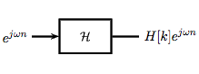
Since complex exponentials (Section 1.8) are eigenfunctions of linear time-invariant (LTI) systems (Section 14.5), calculating the output of an LTI system \(\mathscr{H}\) given \(e^{j \omega n}\) as an input amounts to simple multiplication, where \(\omega_0 = \frac{2 \pi k}{N}\), and where \(H[k] \in \mathbb{C}\) is the eigenvalue corresponding to \(k\). As shown in the figure, a simple exponential input would yield the output
\[y[n]=H[k] e^{j \omega n} \nonumber \]
Using this and the fact that \(\mathscr{H}\) is linear, calculating \(y[n]\) for combinations of complex exponentials is also straightforward.
\[\begin{array}{c}
c_{1} e^{j \omega_{1} n}+c_{2} e^{j \omega_{2} n} \rightarrow c_{1} H\left[k_{1}\right] e^{j \omega_{1} n}+c_{2} H\left[k_{2}\right] e^{j \omega_{1} n} \\
\sum_{l} c_{l} e^{j \omega_{1} n} \rightarrow \sum_{l} c_{l} H\left[k_{l}\right] e^{j \omega_{l} n}
\end{array} \nonumber \]
The action of \(H\) on an input such as those in the two equations above is easy to explain. \(\mathscr{H}\) independently scales each exponential component \(e^{j \omega_l n}\) by a different complex number \(H\left[k_{l}\right] \in \mathbb{C}\). As such, if we can write a function \(y[n]\) as a combination of complex exponentials it allows us to easily calculate the output of a system.
DTFS synthesis
It can be demonstrated that an arbitrary Discrete Time-periodic function \(f[n]\) can be written as a linear combination of harmonic complex sinusoids
\[f[n]=\sum_{k=0}^{N-1} c_{k} e^{j \omega_{0} k n} \label{7.3} \]
where \(\omega_0=\frac{2\pi}{N}\) is the fundamental frequency. For almost all \(f[n]\) of practical interest, there exists \(c_n\) to make Equation \ref{7.3} true. If \(f[n]\) is finite energy (\(f[n] \in L^{2}[0, N]\)), then the equality in Equation \ref{7.3} holds in the sense of energy convergence; with discrete-time signals, there are no concerns for divergence as there are with continuous-time signals.
The \(c_n\) - called the Fourier coefficients - tell us "how much" of the sinusoid \(e^{j \omega_{0} k n}\) is in \(f[n]\). The formula shows \(f[n]\) as a sum of complex exponentials, each of which is easily processed by an LTI system (since it is an eigenfunction of every LTI system). Mathematically, it tells us that the set of complex exponentials \(\left\{\forall k, k \in \mathbb{Z}:\left(e^{j \omega_{0} k n}\right)\right\}\) form a basis for the space of N-periodic discrete time functions.
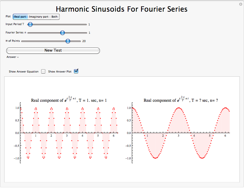
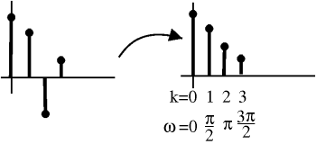
DFT Synthesis Demonstration
DTFS Analysis
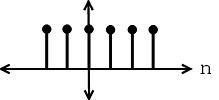
Say we have the following set of numbers that describe a periodic, discrete-time signal, where \(N=4\):
\[\{\ldots, 3,2,-2,1,3, \ldots\} \nonumber \]
Such a periodic, discrete-time signal (with period \(N\)) can be thought of as a finite set of numbers. For example, we can represent this signal as either a periodic signal or as just a single interval as follows:
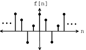 (a)
(a)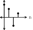 (b)
(b)Note
The cardinalsity of the set of discrete time signals with period \(N\) equals \(\mathbb{C}^N\).
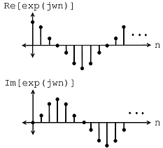
Here, we are going to form a basis using harmonic sinusoids. Before we look into this, it will be worth our time to look at the discrete-time, complex sinusoids in a little more detail.
Complex Sinusoids
If you are familiar with the basic sinusoid signal and with complex exponentials (Section 1.8) then you should not have any problem understanding this section. In most texts, you will see the the discrete-time, complex sinusoid noted as:
\[ e^{j \omega n} \nonumber \]
In the Complex Plane
The complex sinusoid can be directly mapped onto our complex plane, which allows us to easily visualize changes to the complex sinusoid and extract certain properties. The absolute value of our complex sinusoid has the following characteristic:
\[\left|e^{j \omega n}\right|=1, n \in \mathbb{R} \nonumber \]
which tells that our complex sinusoid only takes values on the unit circle. As for the angle, the following statement holds true:
\[\angle\left(e^{j \omega n}\right)=w n \nonumber \]
For more information, see the section on the Discrete Time Complex Exponential to learn about Aliasing, Negative Frequencies, and the formal definition of the Complex Conjugate .
Now that we have looked over the concepts of complex sinusoids, let us turn our attention back to finding a basis for discrete-time, periodic signals. After looking at all the complex sinusoids, we must answer the question of which discrete-time sinusoids do we need to represent periodic sequences with a period \(N\).
Equivalent Question
Find a set of vectors \(\forall n, n=\{0, \ldots, N-1\}:\left(b_{k}=e^{j \omega_{k} n}\right)\) such that \({b_k}\) are a basis for \(\mathbb{C}^n\)
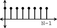
In answer to the above question, let us try the "harmonic" sinusoids with a fundamental frequency \(\omega_{0}=\frac{2 \pi}{N}\):
Harmonic Sinusoid
\[e^{j \frac{2 \pi}{N} k n} \nonumber \]
 (a)
(a)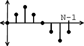 (b)
(b)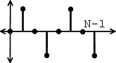 (c)
(c)\(e^{j\frac{2\pi}{N}kn}\) is periodic with period \(N\) and has \(k\) "cycles" between \(n=0\) and \(n=N−1\).
Theorem \(\PageIndex{1}\)
If we let
\[b_{k}[n]=\frac{1}{\sqrt{N}} e^{j \frac{2\pi}{N} k n}, \quad n=\{0, \ldots, N-1\} \nonumber \]
where the exponential term is a vector in \(\mathbb{C}^N\), then \(\left.\left\{b_{k}\right\}\right|_{k=\{0, \ldots, N-1\}}\) is an orthonormal basis (Section 15.8) for \(\mathbb{C}^N\).
Proof
First of all, we must show \({bk}\) is orthonormal, i.e. \(\langle b_{k}, b_{l}\rangle=\delta_{k l}\)
\[\langle b_{k}, b_{l} \rangle=\sum_{n=0}^{N-1} b_{k}[n] b_{l}[n]^{*}=\frac{1}{N} \sum_{n=0}^{N-1} e^{j \frac{2 \pi}{N} k n} e^{-\left(j \frac{2 \pi}{N} l n\right)} \nonumber \]
\[\langle b_{k}, b_{l}\rangle=\frac{1}{N} \sum_{n=0}^{N-1} e^{j \frac{2 \pi}{N}(l-k) n} \nonumber \]
If \(l=k\), then
\[\begin{align}
\left\langle b_{k}, b_{l}\right\rangle &=\frac{1}{N} \sum_{n=0}^{N-1} 1 \nonumber \\
&=1
\end{align} \nonumber \]
If \(l \neq k\) then we must use the "partial summation formula" shown below:
\[\sum_{n=0}^{N-1} \alpha^{n}=\sum_{n=0}^{\infty} \alpha^{n}-\sum_{n=N}^{\infty} \alpha^{n}=\frac{1}{1-\alpha}-\frac{\alpha^{N}}{1-\alpha}=\frac{1-\alpha^{N}}{1-\alpha} \nonumber \]
\[\langle b_{k}, b_{l}\rangle=\frac{1}{N} \sum_{n=0}^{N-1} e^{j \frac{2 \pi}{N}(l-k) n} \nonumber \]
where in the above equation we can say that \(\alpha=e^{j \frac{2 \pi}{N}(l-k)}\), and thus we can see how this is in the form needed to utilize our partial summation formula.
\[ \langle b_{k}, b_{l}\rangle=\frac{1}{N} \frac{1-e^{j \frac{2 \pi}{N}(l-k) N}}{1-e^{j \frac{2 \pi}{N}(l-k)}}=\frac{1}{N} \frac{1-1}{1-e^{j \frac{2 \pi}{N}(l-k)}}=0\nonumber \]
So,
\[\langle b_{k}, b_{l}\rangle=\left\{\begin{array}{ll}
1 & \text { if } k=l \\
0 & \text { if } k \neq l
\end{array}\right. \nonumber \]
Therefore: \({b_k}\) is an orthonormal set. \({b_k}\) is also a basis (Section 14.1), since there are \(N\) vectors which are linearly independent (Section 14.1 - Linear Independence) (orthogonality implies linear independence).
And finally, we have shown that the harmonic sinusoids \(\left\{\frac{1}{\sqrt{N}} e^{j \frac{2 \pi}{N} k n}\right\}\) form an orthonormal basis for \(\mathbb{C}^n\)
Periodic Extension to DTFS
Now that we have an understanding of the discrete-time Fourier series (DTFS), we can consider the periodic extension of \(c[k]\) (the Discrete-time Fourier coefficients). Figure \(\PageIndex{7}\) shows a simple illustration of how we can represent a sequence as a periodic signal mapped over an infinite number of intervals.
 (a)
(a)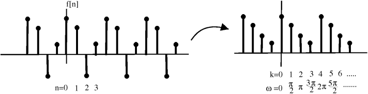 (b)
(b)
Exercise \(\PageIndex{1}\)
Why does a periodic (Section 6.1) extension to the DTFS coefficients \(c[k]\) make sense?
- Answer
-
Aliasing: \(b_k = e^{j\frac{2\pi}{N} kn}\)
\[\begin{align}
b_{k+N} &=e^{j \frac{2 \pi}{N}(k+N) n} \nonumber \\
&=e^{j \frac{2 \pi}{N} k n} e^{j 2 \pi n} \nonumber \\
&=e^{j \frac{2 \pi}{N} n} \nonumber \\
&=b_{k}
\end{align} \nonumber \]
Examples
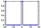
Example \(\PageIndex{1}\): Discrete Time Square Wave
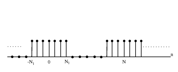
Figure \(\PageIndex{8}\)
the DTFS \(c[k]\) using:
\[c[k]=\frac{1}{N} \sum_{n=0}^{N-1} f[n] e^{-\left(j \frac{2 \kappa}{N} k n\right)} \nonumber \]
Just like continuous time Fourier series, we can take the summation over any interval, so we have
\[c_{k}=\frac{1}{N} \sum_{n=-N_{1}}^{N_{1}} e^{-\left(j \frac{2 \pi}{N} k n\right)} \nonumber \]
Let \(m=n+N_1\) (so we can get a geometric series starting at 0)
\[\sum_{n=0}^{M} a^{n}=\frac{1-a^{M+1}}{1-a} \nonumber \]
\[\begin{align}
c_{k} &=\frac{1}{N} e^{j \frac{2 \pi}{N} N_{1} k} \sum_{m=0}^{2 N_{1}}\left(e^{-\left(j \frac{2 r}{N} k\right)}\right)^{m} \nonumber \\
&=\frac{1}{N} e^{j \frac{2 \pi}{N} N_{1} k} \frac{\left.1-e^{-\left(j \frac{2 \pi}{N}\left(2 N_{1}+1\right)\right.}\right)}{1-e^{-\left(j k \frac{2 \pi}{N}\right)}}
\end{align} \nonumber \]
Now, using the "partial summation formula"
\[\sum_{n=0}^{M} a^{n}=\frac{1-a^{M+1}}{1-a} \nonumber \]
\[\begin{align}
c_{k} &=\frac{1}{N} e^{j \frac{2 \pi}{N} N_{1} k} \sum_{m=0}^{2 N_{1}}\left(e^{-\left(j \frac{2 \pi}{N} k\right)}\right)^{m} \nonumber \\
&=\frac{1}{N} e^{j \frac{2 \pi}{N} N_{1} k} \frac{\left.1-e^{-\left(j \frac{2 \pi}{N}\left(2 N_{1}+1\right)\right.}\right)}{1-e^{-\left(j k \frac{2 \pi}{N}\right)}}
\end{align} \nonumber \]
Manipulate to make this look like a sinc function (distribute):
\[\begin{align}
c_{k} &=\frac{1}{N} \frac{e^{-\left(j k \frac{2 \pi}{2 N}\right)}\left(e^{j k \frac{2 \pi}{N}\left(N_{1}+\frac{1}{2}\right)}-e^{-\left(j k \frac{2 \pi}{N}\left(N_{1}+\frac{1}{2}\right)\right)}\right)}{e^{-\left(j k \frac{2 \pi}{2 N}\right)}\left(e^{j k \frac{2 \pi}{N} \frac{1}{2}}-e^{-\left(j k \frac{2 \pi}{N} \frac{1}{2}\right)}\right)} \nonumber \\
&=\frac{1}{N} \frac{\sin \left(\frac{2 \pi k\left(N_{1}+\frac{1}{2}\right)}{N}\right)}{\sin \left(\frac{\pi k}{N}\right)} \nonumber \\
&=\text { digital sinc }
\end{align} \nonumber \]
Note
It's periodic! Figure \(\PageIndex{9}\), Figure \(\PageIndex{10}\), and Figure \(\PageIndex{11}\) how our above function and coefficients for various values of \(N_1\).
 (a)
(a)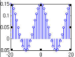 (b)
(b)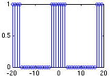 (a)
(a)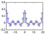 (b)
(b)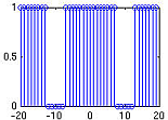 (a)
(a)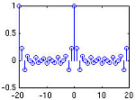 (b)
(b)DTFS conclusion
Using the steps shown above in the derivation and our previous understanding of Hilbert Spaces (Section 15.4) and Orthogonal Expansions (Section 15.9), the rest of the derivation is automatic. Given a discrete-time, periodic signal (vector in \(\mathbb{C}^n\)) \(f[n]\), we can write:
\[f[n]=\frac{1}{\sqrt{N}} \sum_{k=0}^{N-1} c_{k} e^{j \frac{2 \pi}{w} k n} \nonumber \]
\[c_{k}=\frac{1}{\sqrt{N}} \sum_{n=0}^{N-1} f[n] e^{-(j \frac{2\pi}{N}k n)} \nonumber \]
Note: Most people collect both the \(\frac{1}{\sqrt{N}}\) terms into the expression for \(c_k\).
Discrete Time Fourier Series
Here is the common form of the DTFS with the above note taken into account:
\[f[n]=\sum_{k=0}^{N-1} c_{k} e^{j \frac{2 \pi}{N} k n} \nonumber \]
\[c_{k}=\frac{1}{N} \sum_{n=0}^{N-1} f[n] e^{-\left(j \frac{2 \pi}{N} k n\right)} \nonumber \]
This is what the \(\texttt{fft}\) command in MATLAB does.