11.1: Laplace Transform
- Page ID
- 22907
\( \newcommand{\vecs}[1]{\overset { \scriptstyle \rightharpoonup} {\mathbf{#1}} } \)
\( \newcommand{\vecd}[1]{\overset{-\!-\!\rightharpoonup}{\vphantom{a}\smash {#1}}} \)
\( \newcommand{\id}{\mathrm{id}}\) \( \newcommand{\Span}{\mathrm{span}}\)
( \newcommand{\kernel}{\mathrm{null}\,}\) \( \newcommand{\range}{\mathrm{range}\,}\)
\( \newcommand{\RealPart}{\mathrm{Re}}\) \( \newcommand{\ImaginaryPart}{\mathrm{Im}}\)
\( \newcommand{\Argument}{\mathrm{Arg}}\) \( \newcommand{\norm}[1]{\| #1 \|}\)
\( \newcommand{\inner}[2]{\langle #1, #2 \rangle}\)
\( \newcommand{\Span}{\mathrm{span}}\)
\( \newcommand{\id}{\mathrm{id}}\)
\( \newcommand{\Span}{\mathrm{span}}\)
\( \newcommand{\kernel}{\mathrm{null}\,}\)
\( \newcommand{\range}{\mathrm{range}\,}\)
\( \newcommand{\RealPart}{\mathrm{Re}}\)
\( \newcommand{\ImaginaryPart}{\mathrm{Im}}\)
\( \newcommand{\Argument}{\mathrm{Arg}}\)
\( \newcommand{\norm}[1]{\| #1 \|}\)
\( \newcommand{\inner}[2]{\langle #1, #2 \rangle}\)
\( \newcommand{\Span}{\mathrm{span}}\) \( \newcommand{\AA}{\unicode[.8,0]{x212B}}\)
\( \newcommand{\vectorA}[1]{\vec{#1}} % arrow\)
\( \newcommand{\vectorAt}[1]{\vec{\text{#1}}} % arrow\)
\( \newcommand{\vectorB}[1]{\overset { \scriptstyle \rightharpoonup} {\mathbf{#1}} } \)
\( \newcommand{\vectorC}[1]{\textbf{#1}} \)
\( \newcommand{\vectorD}[1]{\overrightarrow{#1}} \)
\( \newcommand{\vectorDt}[1]{\overrightarrow{\text{#1}}} \)
\( \newcommand{\vectE}[1]{\overset{-\!-\!\rightharpoonup}{\vphantom{a}\smash{\mathbf {#1}}}} \)
\( \newcommand{\vecs}[1]{\overset { \scriptstyle \rightharpoonup} {\mathbf{#1}} } \)
\( \newcommand{\vecd}[1]{\overset{-\!-\!\rightharpoonup}{\vphantom{a}\smash {#1}}} \)
\(\newcommand{\avec}{\mathbf a}\) \(\newcommand{\bvec}{\mathbf b}\) \(\newcommand{\cvec}{\mathbf c}\) \(\newcommand{\dvec}{\mathbf d}\) \(\newcommand{\dtil}{\widetilde{\mathbf d}}\) \(\newcommand{\evec}{\mathbf e}\) \(\newcommand{\fvec}{\mathbf f}\) \(\newcommand{\nvec}{\mathbf n}\) \(\newcommand{\pvec}{\mathbf p}\) \(\newcommand{\qvec}{\mathbf q}\) \(\newcommand{\svec}{\mathbf s}\) \(\newcommand{\tvec}{\mathbf t}\) \(\newcommand{\uvec}{\mathbf u}\) \(\newcommand{\vvec}{\mathbf v}\) \(\newcommand{\wvec}{\mathbf w}\) \(\newcommand{\xvec}{\mathbf x}\) \(\newcommand{\yvec}{\mathbf y}\) \(\newcommand{\zvec}{\mathbf z}\) \(\newcommand{\rvec}{\mathbf r}\) \(\newcommand{\mvec}{\mathbf m}\) \(\newcommand{\zerovec}{\mathbf 0}\) \(\newcommand{\onevec}{\mathbf 1}\) \(\newcommand{\real}{\mathbb R}\) \(\newcommand{\twovec}[2]{\left[\begin{array}{r}#1 \\ #2 \end{array}\right]}\) \(\newcommand{\ctwovec}[2]{\left[\begin{array}{c}#1 \\ #2 \end{array}\right]}\) \(\newcommand{\threevec}[3]{\left[\begin{array}{r}#1 \\ #2 \\ #3 \end{array}\right]}\) \(\newcommand{\cthreevec}[3]{\left[\begin{array}{c}#1 \\ #2 \\ #3 \end{array}\right]}\) \(\newcommand{\fourvec}[4]{\left[\begin{array}{r}#1 \\ #2 \\ #3 \\ #4 \end{array}\right]}\) \(\newcommand{\cfourvec}[4]{\left[\begin{array}{c}#1 \\ #2 \\ #3 \\ #4 \end{array}\right]}\) \(\newcommand{\fivevec}[5]{\left[\begin{array}{r}#1 \\ #2 \\ #3 \\ #4 \\ #5 \\ \end{array}\right]}\) \(\newcommand{\cfivevec}[5]{\left[\begin{array}{c}#1 \\ #2 \\ #3 \\ #4 \\ #5 \\ \end{array}\right]}\) \(\newcommand{\mattwo}[4]{\left[\begin{array}{rr}#1 \amp #2 \\ #3 \amp #4 \\ \end{array}\right]}\) \(\newcommand{\laspan}[1]{\text{Span}\{#1\}}\) \(\newcommand{\bcal}{\cal B}\) \(\newcommand{\ccal}{\cal C}\) \(\newcommand{\scal}{\cal S}\) \(\newcommand{\wcal}{\cal W}\) \(\newcommand{\ecal}{\cal E}\) \(\newcommand{\coords}[2]{\left\{#1\right\}_{#2}}\) \(\newcommand{\gray}[1]{\color{gray}{#1}}\) \(\newcommand{\lgray}[1]{\color{lightgray}{#1}}\) \(\newcommand{\rank}{\operatorname{rank}}\) \(\newcommand{\row}{\text{Row}}\) \(\newcommand{\col}{\text{Col}}\) \(\renewcommand{\row}{\text{Row}}\) \(\newcommand{\nul}{\text{Nul}}\) \(\newcommand{\var}{\text{Var}}\) \(\newcommand{\corr}{\text{corr}}\) \(\newcommand{\len}[1]{\left|#1\right|}\) \(\newcommand{\bbar}{\overline{\bvec}}\) \(\newcommand{\bhat}{\widehat{\bvec}}\) \(\newcommand{\bperp}{\bvec^\perp}\) \(\newcommand{\xhat}{\widehat{\xvec}}\) \(\newcommand{\vhat}{\widehat{\vvec}}\) \(\newcommand{\uhat}{\widehat{\uvec}}\) \(\newcommand{\what}{\widehat{\wvec}}\) \(\newcommand{\Sighat}{\widehat{\Sigma}}\) \(\newcommand{\lt}{<}\) \(\newcommand{\gt}{>}\) \(\newcommand{\amp}{&}\) \(\definecolor{fillinmathshade}{gray}{0.9}\)Introduction
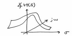
The Laplace transform is a generalization of the Continuous-Time Fourier Transform (Section 8.2). It is used because the CTFT does not converge/exist for many important signals, and yet it does for the Laplace-transform (e.g., signals with infinite \(l_2\) norm). It is also used because it is notationaly cleaner than the CTFT. However, instead of using complex exponentials (Section 7.2) of the form \(e^{j \omega t}\), with purely imaginary parameters, the Laplace transform uses the more general, \(e^{st}\), where \(s=\sigma+j \omega\) is complex, to analyze signals in terms of exponentially weighted sinusoids.
The Laplace Transform
Bilateral Laplace Transform Pair
Although Laplace transforms are rarely solved in practice using integration (tables (Section 11.2) and computers (e.g. Matlab) are much more common), we will provide the bilateral Laplace transform pair here for purposes of discussion and derivation. These define the forward and inverse Laplace transformations. Notice the similarities between the forward and inverse transforms. This will give rise to many of the same symmetries found in Fourier analysis (Section 5.1).
Laplace Transform
\[F(s)=\int_{-\infty}^{\infty} f(t) e^{-(s t)} d t \nonumber \]
Inverse Laplace Transform
\[f(t)=\frac{1}{2 \pi j} \int_{c-j \infty}^{c+j \infty} F(s) e^{s t} d s \nonumber \]
Note
We have defined the bilateral Laplace transform. There is also a unilateral Laplace transform ,
\[F(s)=\int_{0}^{\infty} f(t) e^{-(s t)} \mathrm{d} t \nonumber \]
which is useful for solving the difference equations with nonzero initial conditions. This is similar to the unilateral Z Transform in Discrete time.
Relation between Laplace and CTFT
Taking a look at the equations describing the Z-Transform and the Discrete-Time Fourier Transform:
Continuous-Time Fourier Transform
\[\mathcal{F}(\Omega)=\int_{-\infty}^{\infty} f(t) e^{-(j \Omega t)} d t \nonumber \]
Laplace Transform
\[F(s)=\int_{-\infty}^{\infty} f(t) e^{-(s t)} d t \nonumber \]
We can see many similarities; first, that :
\[\mathcal{F}(\Omega)=F(s) \nonumber \]
for all \(\Omega = s\).
Note
The CTFT is a complex-valued function of a real-valued variable \(\omega\) (and \(2\pi\) periodic). The Z-transform is a complex-valued function of a complex valued variable z.
Plots
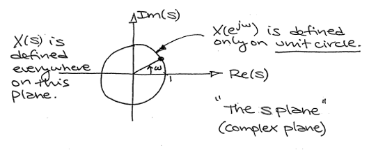
Figure \(\PageIndex{1}\)
Visualizing the Laplace Transform
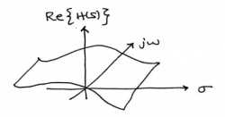
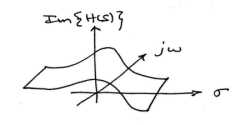
With the Fourier transform, we had a complex-valued function of a purely imaginary variable, \(F(j \omega)\). This was something we could envision with two 2-dimensional plots (real and imaginary parts or magnitude and phase). However, with Laplace, we have a complex-valued function of a complex variable. In order to examine the magnitude and phase or real and imaginary parts of this function, we must examine 3-dimensional surface plots of each component.
Real and imaginary sample plots


Magnitude and phase sample plots


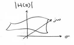
While these are legitimate ways of looking at a signal in the Laplace domain, it is quite difficult to draw and/or analyze. For this reason, a simpler method has been developed. Although it will not be discussed in detail here, the method of Poles and Zeros is much easier to understand and is the way both the Laplace transform and its discrete-time counterpart the Z-transform are represented graphically.
Using a Computer to find the Laplace Transform
Using a computer to find Laplace transforms is relatively painless. Matlab has two functions, laplace
and ilaplace
, that are both part of the symbolic toolbox, and will find the Laplace and inverse Laplace transforms respectively. This method is generally preferred for more complicated functions. Simpler and more contrived functions are usually found easily enough by using tables.
Laplace Transform Definition Demonstration

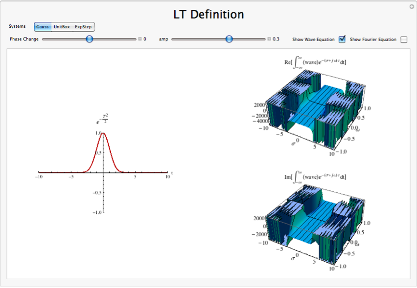
Interactive Demonstrations
Conclusion
The laplace transform proves a useful, more general form of the Continuous Time Fourier Transform. It applies equally well to describing systems as well as signals using the eigenfunction method, and to describing a larger class of signals better described using the pole-zero method.