11.5: Poles and Zeros in the S-Plane

Introduction to Poles and Zeros of the Laplace-Transform

It is quite difficult to qualitatively analyze the Laplace transform (Section 11.1) and Z-transform, since mappings of their magnitude and phase or real part and imaginary part result in multiple mappings of 2-dimensional surfaces in 3-dimensional space. For this reason, it is very common to examine a plot of a transfer function's poles and zeros to try to gain a qualitative idea of what a system does.

Once the Laplace-transform of a system has been determined, one can use the information contained in function's polynomials to graphically represent the function and easily observe many defining characteristics. The Laplace-transform will have the below structure, based on Rational Functions (Section 12.7):

\[H(s)=\frac{P(s)}{Q(s)} \nonumber \]

The two polynomials, \(P(s)\) and \(Q(s)\), allow us to find the poles and zeros of the Laplace-Transform.

Definition: zeros

1. The value(s) for ss where \(P(s)=0\).
2. The complex frequencies that make the overall gain of the filter transfer function zero.

Definition: poles

1. The value(s) for \(s\) where \(Q(s)=0\).
2. The complex frequencies that make the overall gain of the filter transfer function infinite.

Example \(\PageIndex{1}\)

Below is a simple transfer function with the poles and zeros shown below it.

\[H(s)=\frac{s+1}{\left(s-\frac{1}{2}\right)\left(s+\frac{3}{4}\right)} \nonumber \]

The zeros are: \(\{-1\}\)

The poles are: \(\left\{\frac{1}{2},-\frac{3}{4}\right\}\)

The S-Plane

Once the poles and zeros have been found for a given Laplace Transform, they can be plotted onto the S-Plane. The S-plane is a complex plane with an imaginary and real axis referring to the complex-valued variable \(z\). The position on the complex plane is given by \(re^{j \theta}\) and the angle from the positive, real axis around the plane is denoted by \(\theta\). When mapping poles and zeros onto the plane, poles are denoted by an "x" and zeros by an "o". The below figure shows the S-Plane, and examples of plotting zeros and poles onto the plane can be found in the following section.

S-Plane

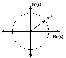
Figure \(\PageIndex{1}\)

Examples of Pole/Zero Plots

This section lists several examples of finding the poles and zeros of a transfer function and then plotting them onto the S-Plane.

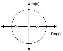
Example \(\PageIndex{2}\): Simple Pole/Zero Plot

\[H(s)=\frac{s}{\left(s-\frac{1}{2}\right)\left(s+\frac{3}{4}\right)} \nonumber \]

The zeros are: \(\{0\}\)

The poles are: \(\left\{\frac{1}{2},-\frac{3}{4}\right\}\)

Pole/Zero Plot

Figure \(\PageIndex{2}\): Using the zeros and poles found from the transfer function, the one zero is mapped to zero and the two poles are placed at \(\frac{1}{2}\) and \(−\frac{3}{4}\)

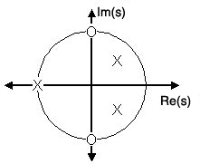
Example \(\PageIndex{3}\): Complex Pole/Zero Plot

\[H(s)=\frac{(s-j)(s+j)}{\left(s-\left(\frac{1}{2}-\frac{1}{2} j\right)\right)\left(s-\frac{1}{2}+\frac{1}{2} j\right)} \nonumber \]

The zeros are: \(\{j,-j\}\)

The poles are: \(\left\{-1, \frac{1}{2}+\frac{1}{2} j, \frac{1}{2}-\frac{1}{2} j\right\}\)

Pole/Zero Plot

Figure \(\PageIndex{3}\): Using the zeros and poles found from the transfer function, the zeros are mapped to \(\pm(j)\), and the poles are placed at \(−1\), \(\frac{1}{2}+\frac{1}{2} j\), and \(\frac{1}{2}-\frac{1}{2} j\)

Example \(\PageIndex{4}\): Pole-Zero Cancellation

An easy mistake to make with regards to poles and zeros is to think that a function like \(\frac{(s+3)(s-1)}{s-1}\) is the same as \(s+3\). In theory they are equivalent, as the pole and zero at \(s=1\) cancel each other out in what is known as pole-zero cancellation. However, think about what may happen if this were a transfer function of a system that was created with physical circuits. In this case, it is very unlikely that the pole and zero would remain in exactly the same place. A minor temperature change, for instance, could cause one of them to move just slightly. If this were to occur a tremendous amount of volatility is created in that area, since there is a change from infinity at the pole to zero at the zero in a very small range of signals. This is generally a very bad way to try to eliminate a pole. A much better way is to use control theory to move the pole to a better place.

Note: Repeated Poles and Zeros

It is possible to have more than one pole or zero at any given point. For instance, the discrete-time transfer function \(H(z)=z^2\) will have two zeros at the origin and the continuous-time function \(H(s)=\frac{1}{s^{25}}\) will have 25 poles at the origin.

MATLAB - If access to MATLAB is readily available, then you can use its functions to easily create pole/zero plots. Below is a short program that plots the poles and zeros from the above example onto the Z-Plane.

	
	% Set up vector for zeros
	z = [j ; -j];

	% Set up vector for poles
	p = [-1 ; .5+.5j ; .5-.5j];

	figure(1);
	zplane(z,p);
	title('Pole/Zero Plot for Complex Pole/Zero Plot Example');
	
      

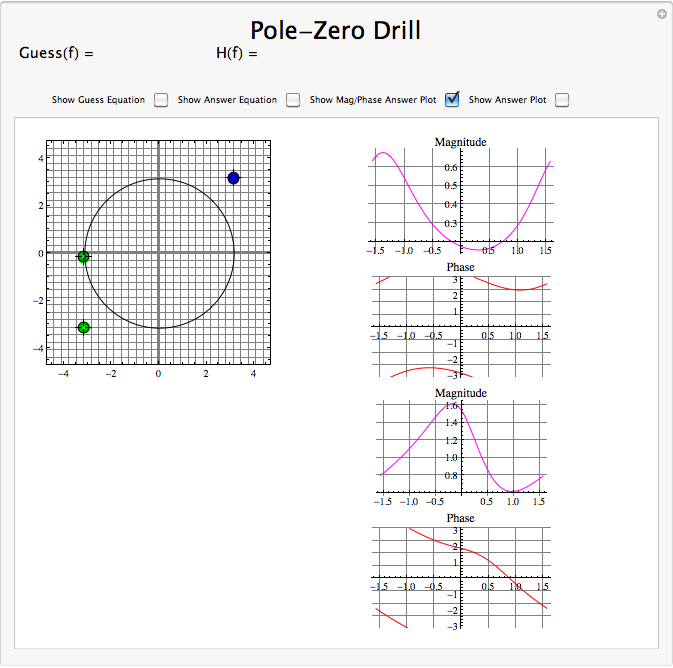
Interactive Demonstration of Poles and Zeros

Figure \(\PageIndex{4}\): Interact (when online) with a Mathematica CDF demonstrating Pole/Zero Plots. To Download, right-click and save target as .cdf.

Applications for pole-zero plots

Stability and Control theory

Now that we have found and plotted the poles and zeros, we must ask what it is that this plot gives us. Basically what we can gather from this is that the magnitude of the transfer function will be larger when it is closer to the poles and smaller when it is closer to the zeros. This provides us with a qualitative understanding of what the system does at various frequencies and is crucial to the discussion of stability (Section 3.6).

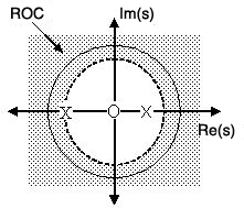
Pole/Zero Plots and the Region of Convergence

The region of convergence (ROC) for \(X(z)\) in the complex Z-plane can be determined from the pole/zero plot. Although several regions of convergence may be possible, where each one corresponds to a different impulse response, there are some choices that are more practical. A ROC can be chosen to make the transfer function causal and/or stable depending on the pole/zero plot.

Filter Properties from ROC

• If the ROC extends outward from the outermost pole, then the system is causal.
• If the ROC includes the unit circle, then the system is stable.

Below is a pole/zero plot with a possible ROC of the Z-transform in the Simple Pole/Zero Plot (Example \(\PageIndex{2}\) discussed earlier. The shaded region indicates the ROC chosen for the filter. From this figure, we can see that the filter will be both causal and stable since the above listed conditions are both met.

Example \(\PageIndex{5}\)

\[H(z)=\frac{z}{\left(z-\frac{1}{2}\right)\left(z+\frac{3}{4}\right)} \nonumber \]

Region of Convergence for the Pole/Zero Plot

Figure \(\PageIndex{5}\): The shaded area represents the chosen ROC for the transfer function.

Frequency Response and Pole/Zero Plots

The reason it is helpful to understand and create these pole/zero plots is due to their ability to help us easily design a filter. Based on the location of the poles and zeros, the magnitude response of the filter can be quickly understood. Also, by starting with the pole/zero plot, one can design a filter and obtain its transfer function very easily.

Conclusion

Pole-Zero Plots are clearly quite useful in the study of the Laplace and Z transform, affording us a method of visualizing the at times confusing mathematical functions.