
14.1: Basic Linear Algebra
- Page ID
- 22928

This brief tutorial on some key terms in linear algebra is not meant to replace or be very helpful to those of you trying to gain a deep insight into linear algebra. Rather, this brief introduction to some of the terms and ideas of linear algebra is meant to provide a little background to those trying to get a better understanding or learn about eigenvectors and eigenfunctions, which play a big role in deriving a few important ideas on Signals and Systems. The goal of these concepts will be to provide a background for signal decomposition and to lead up to the derivation of the Fourier Series.
Linear Independence
A set of vectors \(\left\{x_{1}, x_{2}, \ldots, x_{k}\right\}\) in \(x_{i} \in \mathbb{C}^{n}\) are linearly independent if none of them can be written as a linear combination of the others.
Definition: Linearly Independent
For a given set of vectors, \(\left\{x_{1}, x_{2}, \ldots, x_{n}\right\}\), they are linearly independent if
\[c_{1} x_{1}+c_{2} x_{2}+\dots+c_{n} x_{n}=0 \nonumber \]
only when \(c_{1}=c_{2}=\cdots=c_{n}=0\)
Example \(\PageIndex{1}\)
We are given the following two vectors:
\[\begin{array}{c}
x_{1}=\left(\begin{array}{c}
3 \\
2
\end{array}\right) \\
x_{2}=\left(\begin{array}{c}
-6 \\
-4
\end{array}\right)
\end{array} \nonumber \]
These are not linearly independent as proven by the following statement, which, by inspection, can be seen to not adhere to the definition of linear independence stated above.
\[\left(x_{2}=-2 x_{1}\right) \Rightarrow\left(2 x_{1}+x_{2}=0\right) \nonumber \]
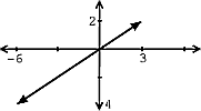
Another approach to reveal a vectors independence is by graphing the vectors. Looking at these two vectors geometrically (as in Figure \(\PageIndex{1}\)), one can again prove that these vectors are not linearly independent.
Example \(\PageIndex{2}\)
We are given the following two vectors:
\[\begin{array}{l}
x_{1}=\left(\begin{array}{l}
3 \\
2
\end{array}\right) \\
x_{2}=\left(\begin{array}{l}
1 \\
2
\end{array}\right)
\end{array} \nonumber \]
These are linearly independent since
\[c_{1} x_{1}=-\left(c_{2} x_{2}\right) \nonumber \]
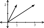
only if \(c_1=c_2=0\). Based on the definition, this proof shows that these vectors are indeed linearly independent. Again, we could also graph these two vectors (see Figure \(\PageIndex{2}\)) to check for linear independence.
Exercise \(\PageIndex{1}\)
Are \(\left\{x_{1}, x_{2}, x_{3}\right\}\) linearly independent?
\[\begin{array}{l}
x_{1}=\left(\begin{array}{l}
3 \\
2
\end{array}\right) \\
x_{2}=\left(\begin{array}{l}
1 \\
2
\end{array}\right) \\
x_{3}=\left(\begin{array}{c}
-1 \\
0
\end{array}\right)
\end{array} \nonumber \]
- Answer
-
By playing around with the vectors and doing a little trial and error, we will discover the following relationship:
\[x_{1}-x_{2}+2 x_{3}=0 \nonumber \]
Thus we have found a linear combination of these three vectors that equals zero without setting the coefficients equal to zero. Therefore, these vectors are not linearly independent!
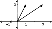
As we have seen in the two above examples, often times the independence of vectors can be easily seen through a graph. However this may not be as easy when we are given three or more vectors. Can you easily tell whether or not these vectors are independent from Figure \(\PageIndex{3}\). Probably not, which is why the method used in the above solution becomes important.
Note
A set of \(m\) vectors in \(\mathbb{C}^{n}\) cannot be linearly independent if \(m>n\).
Span
Definition: Word
The span of a set of vectors \(\left\{x_{1}, x_{2}, \ldots, x_{k}\right\}\) is the set of vectors that can be written as a linear combination of \(\left\{x_{1}, x_{2}, \ldots, x_{k}\right\}\)
\[\operatorname{span}\left(\left\{x_{1}, \ldots, x_{k}\right\}\right)=\left\{\alpha_{1} x_{1}+\alpha_{2} x_{2}+\cdots+\alpha_{k} x_{k}, \quad \alpha_{i} \in \mathbb{C}^{n}\right\} \nonumber \]
Example \(\PageIndex{3}\)
Given the vector
\[x_{1}=\left(\begin{array}{l}
3 \\
2
\end{array}\right) \nonumber \]
the span of \(x_1\) is a line.
Example \(\PageIndex{4}\)
Given the vectors
\[\begin{array}{l}
x_{1}=\left(\begin{array}{l}
3 \\
2
\end{array}\right) \\
x_{2}=\left(\begin{array}{l}
1 \\
2
\end{array}\right)
\end{array}\nonumber \]
the span of these vectors is \(\mathbb{C}^{2}\).
Basis
Definition: Basis
A basis for \(\mathbb{C}^{n}\) is a set of vectors that: (1) spans \(\mathbb{C}^{n}\) and (2) is linearly independent.
Clearly, any set of \(n\) linearly independent vectors is a basis for \(\mathbb{C}^n\).
Example \(\PageIndex{5}\)
We are given the following vector
\[e_{i}=\left(\begin{array}{c}
0 \\
\vdots \\
0 \\
1 \\
0 \\
\vdots \\
0
\end{array}\right) \nonumber \]
where the \(1\) is always in the \(i\)th place and the remaining values are zero. Then the basis for \(\mathbb{C}^n\) is
\[\left\{e_{i}, \quad i=[1,2, \ldots, n]\right\} \nonumber \]
Note
\(\left\{e_{i}, \quad i=[1,2, \ldots, n]\right\}\) is called the standard basis.
Example \(\PageIndex{6}\)
\[\begin{array}{c}
h_{1}=\left(\begin{array}{c}
1 \\
1
\end{array}\right) \\
h_{2}=\left(\begin{array}{c}
1 \\
-1
\end{array}\right)
\end{array} \nonumber \]
\(\left\{h_{1}, h_{2}\right\}\) is a basis for \(\mathbb{C}^2\).
If \(\left\{b_{1}, \ldots, b_{2}\right\}\) is a basis for \(\mathbb{C}^n\), then we can express any \(\boldsymbol{x} \in \mathbb{C}^{n}\) as a linear combination of the \(b_{i}\)'s:
\[x=\alpha_{1} b_{1}+\alpha_{2} b_{2}+\dots+\alpha_{n} b_{n}, \quad \alpha_{i} \in \mathbb{C} \nonumber \]
Example \(\PageIndex{7}\)
Given the following vector,
\[x=\left(\begin{array}{l}
1 \\
2
\end{array}\right) \nonumber \]
writing \(x\) in terms of \(\left\{e_{1}, e_{2}\right\}\) gives us
\[x=e_{1}+2 e_{2} \nonumber \]
Exercise \(\PageIndex{2}\)
Try and write \(x\) in terms of \(\left\{h_{1}, h_{2}\right\}\) (defined in the previous example).
- Answer
-
\[x=\frac{3}{2} h_{1}+\frac{-1}{2} h_{2} \nonumber \]
In the two basis examples above, \(x\) is the same vector in both cases, but we can express it in many different ways (we give only two out of many, many possibilities). You can take this even further by extending this idea of a basis to function spaces.
Note
As mentioned in the introduction, these concepts of linear algebra will help prepare you to understand the Fourier Series, which tells us that we can express periodic functions, \(f(t)\), in terms of their basis functions, \(e^{j \omega_0 nt}\).