14.2: Eigenvectors and Eigenvalues

In this section, our linear systems will be n×n matrices of complex numbers. For a little background into some of the concepts that this module is based on, refer to the basics of linear algebra (Section 14.1).

Eigenvectors and Eigenvalues

Let \(A\) be an \(n \times n\) matrix, where \(A\) is a linear operator on vectors in \(\mathbb{C}^n\).

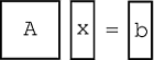
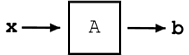
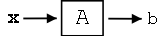
\[Ax=b \label{14.1} \]

where \(x\) and \(b\) are \(n \times 1\) vectors (Figure \(\PageIndex{1}\)).

Figure \(\PageIndex{1}\): Illustration of linear system and vectors.

Definition: Eigenvector

An eigenvector of \(A\) is a vector \(\mathbf{v} \in \mathbb{C}^{n}\) such that

\[A \mathbf{v}=\lambda \mathbf{v} \label{14.2} \]

where \(\lambda\) is called the corresponding eigenvalue. \(A\) only changes the length of \(\mathbf{v}\), not its direction.

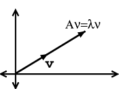
Graphical Model

Through Figure \(\PageIndex{2}\) and Figure \(\PageIndex{3}\), let us look at the difference between Equation \ref{14.1} and Equation \ref{14.2}.

Figure \(\PageIndex{2}\): Represents Equation \ref{14.1}, \(A \mathbf{x}=\mathbf{b}\).

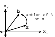
If \(\mathbf{v}\) is an eigenvector of \(A\), then only its length changes. See Figure \(\PageIndex{3}\) and notice how our vector's length is simply scaled by our variable, \(\lambda\), called the eigenvalue:

Figure \(\PageIndex{3}\): Represents Equation \ref{14.2}, \(A \mathbf{v}=\lambda \mathbf{v}\).

Note

When dealing with a matrix \(A\), eigenvectors are the simplest possible vectors to operate on.

Examples

Exercise \(\PageIndex{1}\)

From inspection and understanding of eigenvectors, find the two eigenvectors, \(v_1\) and \(v_2\), of

\[A=\left(\begin{array}{cc}
3 & 0 \\
0 & -1
\end{array}\right) \nonumber \]

Also, what are the corresponding eigenvalues, \(\lambda_1\) and \(\lambda_2\)? Do not worry if you are having problems seeing these values from the information given so far, we will look at more rigorous ways to find these values soon.

Answer

The eigenvectors you found should be:

\[\begin{array}{l}
v_{1}=\left(\begin{array}{l}
1 \\
0
\end{array}\right) \\
v_{2}=\left(\begin{array}{l}
0 \\
1
\end{array}\right)
\end{array} \nonumber \]

And the corresponding eigenvalues are

\[\lambda_1 = 3 \nonumber \]

\[\lambda_2 = -1 \nonumber \]

Exercise \(\PageIndex{2}\)

Show that these two vectors,

\[\begin{array}{l}
v_{1}=\left(\begin{array}{l}
1 \\
1
\end{array}\right) \\
v_{2}=\left(\begin{array}{c}
1 \\
-1
\end{array}\right)
\end{array} \nonumber \]

are eigenvectors of \(A\), where \(A=\left(\begin{array}{cc}
3 & -1 \\
-1 & 3
\end{array}\right)\). Also, find the corresponding eigenvalues.

Answer

In order to prove that these two vectors are eigenvectors, we will show that these statements meet the requirements stated in the definition.

\[\begin{array}{c}
A v_{1}=\left(\begin{array}{cc}
3 & -1 \\
-1 & 3
\end{array}\right)\left(\begin{array}{c}
1 \\
1
\end{array}\right)=\left(\begin{array}{c}
2 \\
2
\end{array}\right) \\
A v_{2}=\left(\begin{array}{cc}
3 & -1 \\
-1 & 3
\end{array}\right)\left(\begin{array}{c}
1 \\
-1
\end{array}\right)=\left(\begin{array}{c}
4 \\
-4
\end{array}\right)
\end{array} \nonumber \]

These results show us that \(A\) only scales the two vectors (i.e. changes their length) and thus it proves that Equation \ref{14.2} holds true for the following two eigenvalues that you were asked to find:

\[\lambda_1 = 2 \nonumber \]

\[\lambda_2 = 4 \nonumber \]

If you need more convincing, then one could also easily graph the vectors and their corresponding product with \(A\) to see that the results are merely scaled versions of our original vectors, \(v_1\) and \(v_2\).

Khan Lecture on Eigenvectors

Figure \(\PageIndex{4}\): video from Khan Academy - Introduction to Eigenvectors and Eigenvalues - 7:43 min.

Calculating Eigenvalues and Eigenvectors

In the above examples, we relied on your understanding of the definition and on some basic observations to find and prove the values of the eigenvectors and eigenvalues. However, as you can probably tell, finding these values will not always be that easy. Below, we walk through a rigorous and mathematical approach at calculating the eigenvalues and eigenvectors of a matrix.

Finding Eigenvalues

Find \(\lambda \in \mathbb{C}\) such that \(\mathbf{v} \neq \mathbf{0}\), where \(\mathbf{0}\) is the "zero vector." We will start with Equation \ref{14.2}, and then work our way down until we find a way to explicitly calculate \(\lambda\).

\[\begin{array}{c}
A \mathbf{v}=\lambda \mathbf{v} \\
A \mathbf{v}-\lambda \mathbf{v}=0 \\
(A-\lambda I) \mathbf{v}=0
\end{array} \nonumber \]

In the previous step, we used the fact that

\[\lambda \mathbf{v}=\lambda I \mathbf{v} \nonumber \]

where \(I\) is the identity matrix.

\[I=\left(\begin{array}{cccc}
1 & 0 & \dots & 0 \\
0 & 1 & \dots & 0 \\
0 & 0 & \ddots & \vdots \\
0 & \dots & \dots & 1
\end{array}\right)\nonumber \]

So, \(A−\lambda I\) is just a new matrix.

Example \(\PageIndex{1}\)

Given the following matrix, \(A\), then we can find our new matrix, \(A−\lambda I\).

\[\begin{array}{c}
A=\left(\begin{array}{cc}
a_{1,1} & a_{1,2} \\
a_{2,1} & a_{2,2}
\end{array}\right) \\
A-\lambda I=\left(\begin{array}{cc}
a_{1,1}-\lambda & a_{1,2} \\
a_{2,1} & a_{2,2}-\lambda
\end{array}\right)
\end{array} \nonumber \]

If \((A−\lambda I) \mathbf{v} = 0\) for some \(\mathbf{v} \neq 0\), then \(A− \lambda I\) is not invertible. This means:

\[\operatorname{det}(A-\lambda I)=0 \nonumber \]

This determinant (shown directly above) turns out to be a polynomial expression (of order \(n\)). Look at the examples below to see what this means.

Example \(\PageIndex{2}\)

Starting with matrix \(A\) (shown below), we will find the polynomial expression, where our eigenvalues will be the dependent variable.

\[A=\left(\begin{array}{cc}
3 & -1 \\
-1 & 3
\end{array}\right) \nonumber \]

\[A-\lambda I=\left(\begin{array}{cc}
3-\lambda & -1 \\
-1 & 3-\lambda
\end{array}\right) \nonumber \]

\[\operatorname{det}(A-\lambda I)=(3-\lambda)^{2}-(-1)^{2}=\lambda^{2}-6 \lambda+8 \nonumber \]

\[\lambda=\{2,4\} \nonumber \]

Example \(\PageIndex{3}\)

Starting with matrix \(A\) (shown below), we will find the polynomial expression, where our eigenvalues will be the dependent variable.

\[\begin{array}{c}
A=\left(\begin{array}{cc}
a_{1,1} & a_{1,2} \\
a_{2,1} & a_{2,2}
\end{array}\right) \\
A-\lambda I=\left(\begin{array}{cc}
a_{1,1}-\lambda & a_{1,2} \\
a_{2,1} & a_{2,2}-\lambda
\end{array}\right) \\
\operatorname{det}(A-\lambda I)=\lambda^{2}-\left(a_{1,1}+a_{2,2}\right) \lambda-a_{2,1} a_{1,2}+a_{1,1} a_{2,2}
\end{array} \nonumber \]

If you have not already noticed it, calculating the eigenvalues is equivalent to calculating the roots of

\[\operatorname{det}(A-\lambda I)=c_{n} \lambda^{n}+c_{n-1} \lambda^{n-1}+\dots+c_{1} \lambda+c_{0}=0 \nonumber \]

Conclusion

Therefore, by simply using calculus to solve for the roots of our polynomial we can easily find the eigenvalues of our matrix.

Finding Eigenvectors

Given an eigenvalue, \(\lambda_i\), the associated eigenvectors are given by

\[\begin{array}{c}
A \mathbf{v}=\lambda_{i} \mathbf{v} \\
A\left(\begin{array}{c}
v_{1} \\
\vdots \\
v_{n}
\end{array}\right)=\left(\begin{array}{c}
\lambda_{1} v_{1} \\
\vdots \\
\lambda_{n} v_{n}
\end{array}\right)
\end{array} \nonumber \]

set of \(n\) equations with \(n\) unknowns. Simply solve the \(n\) equations to find the eigenvectors.

Khan Lecture on Deriving Eigenvectors and Eigenvalues

Figure \(\PageIndex{5}\): video from Khan Academy - Example Deriving Eigenvectors and Eigenvalues - 5:39 min.

Main Point

Say the eigenvectors of \(A\), \(\left\{v_{1}, v_{2}, \ldots, v_{n}\right\}\), span \(\mathbb{C}^n\), meaning \(\left\{v_{1}, v_{2}, \ldots, v_{n}\right\}\) are linearly independent (Section 14.1) and we can write any \(\mathbf{x} \in \mathbb{C}^{n}\) as

\[\mathbf{x}=\alpha_{1} v_{1}+\alpha_{2} v_{2}+\cdots+\alpha_{n} v_{n} \label{14.3} \]

where \(\left\{\alpha_{1}, \alpha_{2}, \ldots, \alpha_{n}\right\} \in \mathrm{C}\). All that we are doing is rewriting \(\mathbf{x}\) in terms of eigenvectors of \(A\). Then,

\[\begin{array}{c}
A \mathbf{x}=A\left(\alpha_{1} v_{1}+\alpha_{2} v_{2}+\cdots+\alpha_{n} v_{n}\right) \\
A \mathbf{x} =\alpha_{1} A v_{1}+\alpha_{2} A v_{2}+\cdots+\alpha_{n} A v_{n} \\
A \mathbf{x} =\alpha_{1} \lambda_{1} v_{1}+\alpha_{2} \lambda_{2} v_{2}+\cdots+\alpha_{n} \lambda_{n} v_{n}=b
\end{array} \nonumber \]

Therefore we can write,

\[\mathbf{x}=\sum_{i} \alpha_{i} v_{i} \nonumber \]

and this leads us to the following depicted system:

Figure \(\PageIndex{6}\): Depiction of system where we break our vector, \(\mathbf{x}\), into a sum of its eigenvectors.

where in Figure \(\PageIndex{6}\) we have,

\[b=\sum_{i} \alpha_{i} \lambda_{i} v_{i} \nonumber \]

Main Point:

By breaking up a vector, \(\mathbf{x}\), into a combination of eigenvectors, the calculation of \(A\mathbf{x}\) is broken into "easy to swallow" pieces.

Practice Problem

Exercise \(\PageIndex{3}\)

For the following matrix, \(A\) and vector, \(\mathbf{x}\), solve for their product. Try solving it using two different methods: directly and using eigenvectors.

\[\begin{aligned}
A &=\left(\begin{array}{cc}
3 & -1 \\
-1 & 3
\end{array}\right) \\
& \mathbf{x}=\left(\begin{array}{l}
5 \\
3
\end{array}\right)
\end{aligned} \nonumber \]

Answer

Direct Method (use basic matrix multiplication)

\[A \mathbf{x}=\left(\begin{array}{cc}
3 & -1 \\
-1 & 3
\end{array}\right)\left(\begin{array}{l}
5 \\
3
\end{array}\right)=\left(\begin{array}{c}
12 \\
4
\end{array}\right) \nonumber \]

Eigenvectors (use the eigenvectors and eigenvalues we found earlier for this same matrix)

\[\begin{array}{c}
v_{1}=\left(\begin{array}{c}
1 \\
1
\end{array}\right) \\
v_{2}=\left(\begin{array}{c}
1 \\
-1
\end{array}\right) \\
\lambda_{1}=2 \\
\lambda_{2}=4
\end{array} \nonumber \]

As shown in Equation \ref{14.3}, we want to represent \(x\) as a sum of its scaled eigenvectors. For this case, we have:

\[\begin{array}{c}
\mathbf{x} = 4 v_{1}+v_{2} \\
\mathbf{x} =\left(\begin{array}{c}
5 \\
3
\end{array}\right)=4\left(\begin{array}{c}
1 \\
1
\end{array}\right)+\left(\begin{array}{c}
1 \\
-1
\end{array}\right) \\
A \mathbf{x} = A\left(4 v_{1}+v_{2}\right)=\lambda_{i}\left(4 v_{1}+v_{2}\right)
\end{array} \nonumber \]

Therefore, we have

\[A \mathbf{x}=4 \times 2\left(\begin{array}{l}
1 \\
1
\end{array}\right)+4\left(\begin{array}{c}
1 \\
-1
\end{array}\right)=\left(\begin{array}{c}
12 \\
4
\end{array}\right) \nonumber \]

Notice that this method using eigenvectors required no matrix multiplication. This may have seemed more complicated here, but just imagine \(A\) being really big, or even just a few dimensions larger!