17.4: A More General Description

There are at least two reasons for going to a more general system description than those shown up to now. First, our assessment of the performance of the system may involve variables that are not among the measured/fed-back output signals of the plant. Second, the disturbances affecting the system may enter in more general ways than indicated previously. We do still want our system representation to separate out the controller portions of the system (the \(K\)'s or \(K_{1}\), \(K_{2}\) of the earlier figures), as these are the portions that we will be designing. In this section we will introduce a general plant description that organizes the different types of inputs and outputs, and their interaction with a controller. A block diagram for a general plant description is shown in Figure 17.6.

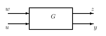
Figure \(\PageIndex{1}\): General plant description.

The different signals in Figure 17.6 can be classified as follows.

Inputs

1. Control input vector \(u\), which contains the actuator signals driving the plant and generated by a controller.
2. Exogeneous input vector \(w\), which contains all other external signals, such as references and disturbances.

Outputs

1. Measured output vector \(y\), which contains the signals that are available to the controller. These are based on the outputs of the sensor devices, and form the input to the controller.
2. Regulated output vector \(z\), which contains the signals that are important for the specific application. The regulated outputs usually include the actuator signals, the tracking error signals, and the state variables that must be manipulated.

Let the transfer function matrix

\[G=\left[\begin{array}{ll}
G_{z w} & G_{z u} \\
G_{y w} & G_{y u}
\end{array}\right]\nonumber\]

have the state-space realization

\[\begin{array}{l}
\dot{x}=A x+B_{1} w+B_{2} u \\
z=C_{1} x+D_{11} w+D_{12} u \\
y=C_{2} x+D_{21} w+D_{22} u
\end{array}\nonumber\]

Example 17.4

Consider the unity feedback system in Figure 17.7, where \(P\) is a SISO plant, \(K\) is a scalar controller, \(y^{\prime}\) is the output, \(u\) is the control input, \(v\) is a reference signal, and \(d\) is an external disturbance that is "shaped" by the filter \(H\) before it is injected into the measured output. The controller is driven by the difference \(e=v-y^{\prime}\) (the "tracking error"). The signals \(v\) and \(d\) can be taken to constitute the exogeneous input, so

\[w=\left[\begin{array}{l}
v \\
d
\end{array}\right]\nonumber\]

In such a configuration we typically want to keep the tracking error \(e\) small, and to put a cost on the control action. We can therefore take the regulated output \(z\) to be

\[z=\left[\begin{array}{l}
e \\
u
\end{array}\right]\nonumber\]

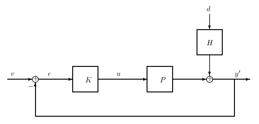
Figure \(\PageIndex{2}\): Example of a unity feedback system.

The input to the controller is \(e\), therefore we set the measured output \(y\) to be equal to \(e\). With these choices, the generalized plant transfer function \(G\), which relates \(z\) and \(y\) to \(w\) and \(u\), can be obtained from

\[\begin{array}{l}
z=\left[\begin{array}{c}
-P u-H d+v \\
u
\end{array}\right]=\left[\begin{array}{c}
-P \\
1
\end{array}\right] u+\left[\begin{array}{cc}
1 & -H \\
0 & 0
\end{array}\right] w \\
y=-P u+\left[\begin{array}{cc}
1 & -H
\end{array}\right] w
\end{array}\nonumber\]

Let us suppose that \(P=\frac{1}{s-1}\) and \(H=\frac{1}{s+1}\). Then a state-space realization of \(G\) is easily obtained:

\[\begin{aligned}
\frac{d}{d t}\left[\begin{array}{c}
x_{1} \\
x_{2}
\end{array}\right] &=\left[\begin{array}{cc}
1 & 0 \\
0 & -1
\end{array}\right]\left[\begin{array}{c}
x_{1} \\
x_{2}
\end{array}\right]+\left[\begin{array}{cc}
0 & 0 \\
0 & 1
\end{array}\right] w+\left[\begin{array}{c}
1 \\
0
\end{array}\right] u \\
z &=\left[\begin{array}{cc}
-1 & -1 \\
0 & 0
\end{array}\right]\left[\begin{array}{c}
x_{1} \\
x_{2}
\end{array}\right]+\left[\begin{array}{cc}
1 & 0 \\
0 & 0
\end{array}\right] w+\left[\begin{array}{c}
0 \\
1
\end{array}\right] u \\
y &=\left[\begin{array}{cc}
-1 & -1
\end{array}\right]\left[\begin{array}{c}
x_{1} \\
x_{2}
\end{array}\right]+\left[\begin{array}{cc}
1 & 0
\end{array}\right] w+0 u
\end{aligned}\nonumber\]

If we close the loop, the general plant/controller structure takes the form shown in Figure 17.8.

The plant transfer matrix \(G\) is a \(2 \times 2\) block matrix mapping the inputs \(w, u\) to the outputs \(z, y\), where the part of the plant that interacts directly with the controller is just \(G_{yu}\). The map (or transfer function) of interest in performance specifications is the map from \(w\) to \(z\), denoted by \(\Phi\), and easily seen to be given by the following expression:

\[\Phi=G_{z w}+G_{z u}\left(I-K G_{y u}\right)^{-1} K G_{y w} \ \tag{17.8}\]

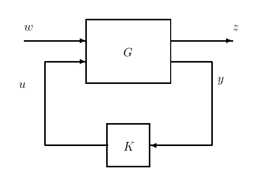
Figure \(\PageIndex{3}\): A general feedback configuration

In this new settup we would like to determine under what conditions the closed-loop system in Figure 17.9 is well-posed and externally stable. For these purposes we inject signals \(r\) and \(v\) as shown in Figure 17.9, which is similar to what we did in the previous sections. Note that by defining the signals

\[\begin{array}{l}
r_{1}=\left(\begin{array}{c}
w \\
r
\end{array}\right) & r_{2}=\left(\begin{array}{c}
0 \\
v
\end{array}\right) \\
y_{1}=\left(\begin{array}{c}
z \\
y
\end{array}\right) & y_{2}=\left(\begin{array}{c}
0 \\
f
\end{array}\right)
\end{array}\nonumber\]

this structure is equivalent to the structure in Figure 17.5. This is illustrated in Figure 17.10, with

\[\begin{array}{l}
H_{1}=\left[\begin{array}{ll}
G_{z w} & G_{z u} \\
G_{y w} & G_{y u}
\end{array}\right] \\
H_{2}=\left[\begin{array}{l}
0 \\
I
\end{array}\right] K\left[\begin{array}{ll}
0 & I
\end{array}\right]=\left[\begin{array}{ll}
0 & 0 \\
0 & K
\end{array}\right]
\end{array}\nonumber\]

This interconnection is well-posed if and only if

\[\left(I-\left(\begin{array}{cc}
G_{z w}(\infty) & G_{z u}(\infty) \\
G_{y w}(\infty) & G_{y u}(\infty)
\end{array}\right)\left(\begin{array}{cc}
0 & 0 \\
0 & K(\infty)
\end{array}\right)\right)\nonumber\]

is invertible. This is the same as requiring that

\[\left(I-K(s) G_{y u}(s)\right)^{-1} \text{ or equivalently } \left(I- G_{y u}(s) K(s)\right)^{-1} \text{ exists and is proper }\nonumber\]

The inputs in Figure 17.9 are related to the signals \(z\), \(u\) and \(y\) as follows:

\[\left[\begin{array}{ccc}
I & -G_{z u} & 0 \\
0 & I & -K \\
0 & -G_{y u} & I
\end{array}\right]\left[\begin{array}{l}
z \\
u \\
y
\end{array}\right]=\left[\begin{array}{ccc}
G_{z w} & 0 & 0 \\
0 & I & K \\
G_{y w} & 0 & 0
\end{array}\right]\left[\begin{array}{l}
w \\
r \\
v
\end{array}\right] \ \tag{17.9}\]

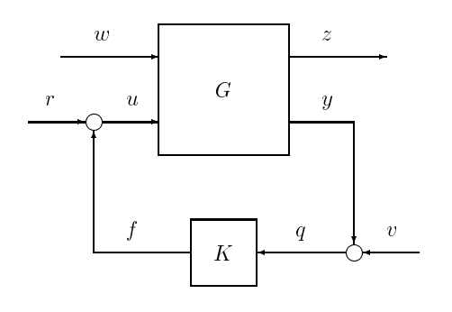
Figure \(\PageIndex{4}\): A more general feedback configuration

Let the map \(\mathcal{T}(P, K)\) be defined as follows:

\[\left(\begin{array}{l}
z \\
u \\
y
\end{array}\right)=\mathcal{T}(P, K)\left(\begin{array}{l}
w \\
r \\
v
\end{array}\right)\nonumber\]

The interconnected system is externally \(p\)-stable if the map from \(r_{1}, r_{2}\) to \(y_{1}, y_{2}\) is \(p\)-stable, see Figure 17.10. This is equivalent to requiring that the map \(\mathcal{T}(P, K)\) is \(p\)-stable.