19.3: The Nyquist Criterion

Before we analyze the stability of feedback loops where the plant is uncertain, we will review the Nyquist criterion. Consider the feedback structure in Figure 19.3. The transfer function

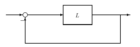
Figure 19.3 : Unity Feedback Confuguration.

\(L\) is called the open-loop transfer function. The condition for the stability of the system in 19.3 is assured if the zeros of \(1 + L\) are all in the left half of the complex plane. The argument principle from complex analysis gives a criterion to calculate the difference between the number of zeros and the number of poles of an analytic function in a certain domain, \(\mathcal{D}\) in the complex plane. Suppose the domain is as shown in Figure 19.4, and the boundary of \(\mathcal{D}\), denoted by \(\delta \mathcal{D}\), is oriented clockwise. We call this oriented boundary of \(\mathcal{D}\) the Nyquist contour.

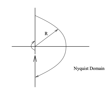
Figure 19.4 : Nyquist Domain.

As the radius of the semicircle in Figure 19.4 goes to infinty the domain covers the right half of the complex plane. The image of \(\delta \mathcal{D}\) under \(L\) is called a Nyquist plot, see Figure 19.5. Note that if \(L\) has poles at the \( j \omega\) axis then we indent the Nyquist contour to avoid these poles, as shown in Figure 19.4. Define

\[\pi_{ol} = \text { Open- loop poles = Number of ploes of L in D = Number of poles of 1 + L in D }\nonumber\]

\[\pi_{el} = \text { Closed- loop poles = Number of zeros of 1 + L in D }\nonumber\]

From the argument principle it follows that

\[\pi_{el} - \pi_{ol}= \text { The number of clockwise encirclements that the Nyquist Plot makes of the point} -1. \nonumber\]

Using this characterization of the difference of the number of the closed-loop poles and the open-loop poles we arrive at the following theorem for the stability of Figure 19.3

Theorem 19.1

The closed-loop system in Figure 19.3 is stable if and only if the Nyquist plot

• does not pass through the origin,
• makes \(\pi_{ol}\) counter-clockwise encirclements of \(-1\).