6.4: Applying lumping to shapes

Lumping by replacing varying quantities with their typical, or characteristic, values is close to the next form of lumping: lumping shapes. Our first illustration is explaining a curious fact about everyday materials.

6.4.1 Densities of liquids and solids

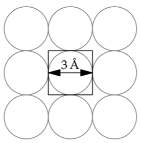
Among books teaching the art of approximation, a classic is Consider a Spherical Cow [22], so named because a sphere is a much simpler shape than a cow. An even simpler shape is a cube. Thus, a powerful form of lumping is to replace complex shapes by a comparably sized cube. With this idea, we can explain why most solids and liquids have densities between 1 and 10 times the density of water.

Each atom is a complex, ill-defined shape, but pretend that it is cube. Because the atoms touch, the density of the substance is approximately the density of one approximating cube:

\[\rho \approx \frac{\textrm{mass of the atom}}{\textrm{volume of the lumped cube}}.\]

To evaluate the numerator, use A as the atom’s atomic mass. Although A is called a mass, it is dimensionless: It is almost exactly the total number of protons and neutrons in the nucleus. Because protons and neutrons have almost the same mass, the proton mass m_p can represent the mass of either constituent. Then the mass of one cube is Am_p.

To find the denominator, the cube’s volume, make each cube’s side be a typical atomic diameter of a ~ 3 ångströms. This size is based on our calculation in Section 5.5.1 of the diameter of the smallest atom, hydrogen (whose diameter was roughly 1 ångström). Then the density becomes

\[\rho \sim \frac{Am_{p}}{(3 \mathring{A})^{3}}.\]

To avoid looking up the proton mass m_p, let’s multiply this fraction by \(N_{A}/N_{A}\), where N_A is Avogadro’s number:

\[\rho \sim \frac{A \times m_{p}N_{A}}{(3 \mathring{A})^{3} \times N_{A}}.\]

The numerator is A grams per mole, because 1 mole of protons (roughly, of hydrogen) has a mass of 1 gram. The denominator is roughly 18 cubic centimeters per mole:

\[\underbrace{3 \times 10^{-23} cm^{3}}_{(3 \mathring{A})^{3}} \times \underbrace{6 \times 10^{23} mol^{-1}}_{N_{A}} = \frac{18 cm^{3}}{mol}.\]

A typical solid or liquid density is then related simply to the substance’s atomic mass A:

\[\rho \sim \frac{A g mol^{-1}}{18 cm^{3} mol^{-1}} = \frac{A}{18} \frac{g}{cm^{3}}.\]

Problem 6.13: Rounding to estimate atomic volume

Use rounding to the nearest half power of ten (Section 6.2.2) to show that a cube with side length 3 ångströms has a volume of approximately 3 × 10⁻²³ cubic centimeters.

Many common elements have atomic masses between 18 and 180, so the densities of many liquids and solids should lie between 1 and 10 grams per cubic centimeter. As shown in the table, the prediction is reasonable. The table even includes a joker: water is not an element! Yet the density estimate is exact.

	A	\(\rho\) (g cm^-3) est.	\(\rho\) (g cm^-3) actual
Li	7	0.4	0.5
H2O	18	1.0	1.0
Si	28	1.6	2.4
Fe	56	3.1	7.9
Hg	201	11.2	13.5
U	238	13.3	18.7
Au	197	10.9	19.3

The table also shows why centimeters and grams are, for materials physics, more convenient than are meters and kilograms. A typical solid has a density of a few grams per cubic centimeter. Such modest numbers are easy to remember and handle. In contrast, a density of 3000 kilograms per cubic meter, although mathematically equivalent, is mentally unwieldy. On each use, you have to think, “How many powers of ten were there again?” Therefore, the table gives densities in the mentally friendly units of grams per cubic centimeter.

Problem 6.14: Accounting for discrepancies in the density prediction

In the table of densities, iron (Fe) shows the biggest discrepancy between the actual and predicted densities, by roughly a factor of 2.5. Use that factor to make an improved estimate for the interatomic spacing in iron.

Problem 6.15: Number density of conduction electrons

Estimate the number density of free (conduction) electrons in a copper wire.

Problem 6.16: Typical drift speed in a wire

a. Use your estimate of the number density of conduction electrons in a copper wire (Problem 6.15) to estimate the drift speed of electrons in the wire connecting a typical lamp to the wall socket.

b. Estimate the time required for electrons to travel at this drift speed from the wall socket to the light bulb. Then how does the light bulb turn on right after you flip the switch?

6.4.2 Graph lumping: The number of undergraduate students

A particularly important shape is a graph. When applied to graphs, the idea of lumping shapes simplifies many a problem, making evident its essential features. As an example of graph lumping, we’ll estimate the number of US undergraduate students. Such back-of-the-envelope market-size estimates are valuable for business planning and for making public policy.

The first step is to estimate the number of people in the United States who are 18, 19, 20, or 21 years old. This total provides, at least in the United States, the pool from which most undergraduate students come. Because not all 18-to-21-year-olds go to college, at the end we will multiply the total by the fraction of adults who are college graduates.

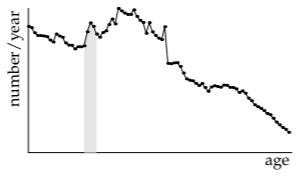
Finding the exact pool size requires the birth date of every person in the United States. Although these data are collected once every decade by the US Census Bureau, they would only overwhelm us. As an approximation to the voluminous data, the Census Bureau also publishes the number of people at each age. For example, the 1991 data are the wiggly line in the graph. The left side of the graph represents the number of infants and toddlers in 1991, and the right side represents the number of older people (also in 1991). The undergraduate pool size, representing all 18-, 19-, 20-, and 21-year-olds, is the shaded area. (The peak around the ages 30–35 represents the baby boomers, born in the period after World War Two.)

Unfortunately, even this graph depends on the huge resources of the Census Bureau, so it is not suited for back-of-the-envelope estimates. It also provides little insight or transfer value. Insight comes from lumping: from turning the complex, wiggly curve into a rectangle. The rectangle’s dimensions can be determined without any information from the Census Bureau.

What are the height and width of this rectangle?

The rectangle’s width is a time, so it must be a characteristic time related to the population. A good guess is the life expectancy, because the age distribution varies significantly overthat time. In the United States, the life expectancy is roughly 75 years, which will be the rectangle’s width. In this lumping approximation, everyone lives happily until a sudden death at his or her 75th birthday. This all-or-nothing reasoning is the essential characteristic of lumping, making it such a useful approximation.

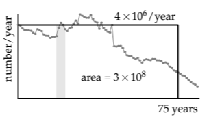
The rectangle’s height can be computed from its area, which is the US population—approximately 300 million (as we estimated in Section 6.3.1). Therefore, the height is 4 million per year:

\[\textrm{height} = \frac{\textrm{area}}{\textrm{width}} \sim \frac{300 \textrm{million}}{75 \textrm{years}} = frac{4 \textrm{million}}{year}.\]

Based on this estimate, there should be 16 million people (in the United States) with the four undergraduate ages of 18, 19, 20, or 21 years.

Not everyone in this pool is an undergraduate. Therefore, the final step is to account for the fraction of adults who are college graduates. In the United States, where education has traditionally been widely spread throughout the population, this fraction (or adjustment factor) is high—say, 0.5. The number of US undergraduates should be about 8 million.

For comparison, the 2010 US census data gives 5.361 million enrolled in four-year colleges, and 4.942 million in two-year colleges, for a combined total of almost exactly 10 million. Our estimate, which lies halfway between the four-year and the combined total, is quite good!

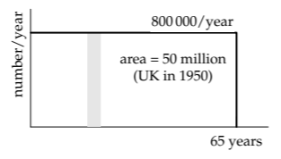
Even had it been terrible, with a large discrepancy between the estimate and the actual number, we would still have learned useful information about a society. As an example, let’s use the same method to estimate how many university students graduated in 1950 in the United Kingdom. (“College” in American English and “university” in British English are roughly equivalent.) The UK population at the time was 50 million. With a life expectancy of, say, 65 years, the rectangle’s height is roughly 800 000 per year. If, as in the United States of today, 50 percent of the age-eligible population goes to university, 400 000 should graduate each year. However, in 1950, the actual number was roughly 17 000—more than a factor of 20 smaller than the estimate.

Such a huge error probably does not come from the population estimate. Instead, the fraction of 50 percent of university participation must be far too high. Indeed, rather than 50 percent, the actual figure for 1950 is 3.4 percent. The difference between 50- and 3-percent university participation makes the United Kingdom of 1950 a very different society from the United States of 2010 or even from the United Kingdom of 2010, where the fraction going to university is roughly 40 percent.

6.4.3 Cone free-fall time and distance

For our next illustration of graph lumping, let’s turn from the social to the physical world, to our falling cones. For the single cone of Section 3.5.2 and the cone race of Section 4.3.1, we assumed that the cones made their entire journey at their terminal speed. But this assumption cannot be exact: Just after the cones are released, their fall speed is zero. Graph lumping will help us evaluate and refine this assumption.

How far does the cone fall before it reaches its terminal speed?

Taken literally, the answer is infinity, because no object reaches its terminal speed. As it approaches its terminal speed, the drag and weight more nearly balance, the force and acceleration get closer to zero, and the speed changes ever more slowly. So an object can approach its terminal speed only ever more closely. Let’s therefore rephrase the question to ask how far the cone falls before it has reached a significant fraction of its terminal speed. In the “significant,” you can see the door through which we will bring in lumping.

Here is a sketch of the actual fall speed versus time. At first, the speed increases rapidly. As the speed increases, so does the drag. The net force and the acceleration fall, so the speed increases more slowly. As a lumping approximation, we’ll replace the smooth curve by a slanted and a horizontal segment.

A partly triangular lumping approximation might look different from the population lumping rectangles we constructed in Section 6.4.2. However, it is merely the integral of a rectangle: It is equivalent to replacing the actual, complicated acceleration by a rectangle representing the period of free fall. Then the acceleration drops abruptly to zero.

Just as we labeled the population rectangle with its height and width, here we label the velocity graph with speeds, times, and slopes. The graph has two segments. The second, horizontal segment shows the cone’s falling at its terminal speed \(v_{term}\). This speed, as we found experimentally in Section 3.5.2, is roughly 1 meter per second.

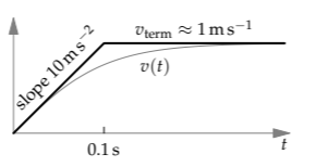
The first, slanted segment represents free fall, as if there were no air resistance. The free-fall acceleration is g, so the free-fall velocity has slope g: In 1 second, the speed increases by 10 meters per second. The slanted and horizontal segments meet where \(gt = v_{term}\). Thus, they meet at approximately 0.1 seconds. Based on the lumping approximation, we expect the cone to reach a significant fraction of its terminal speed by 0.1 seconds—which is only 5 percent of the total fall time of 2 seconds.

Roughly how far does the cone fall in this time?

Use lumping again! The distance is the area of the shaded triangle. The triangle’s base is 0.1 seconds, and its height is the terminal speed, approximately 1 meter per second. So its area is 5 centimeters:

\[\frac{1}{2} \times 0.1 s \times 1 m s^{-1} = 5cm.\]

After only 2.5 percent of its 2-meter journey, the cone has reached a significant fraction of the terminal speed. The “always at terminal speed” approximation is quite accurate. Thanks to the lumping, we could judge the approximation without setting up or solving differential equations.

Problem 6.17: Raindrop terminal speed

Sketch the fall speed of a large raindrop versus time. Roughly how long and how far does it fall before it reaches (a significant fraction of) its terminal speed?

Problem 6.18: Actual cone fall speed

Set up and solve the differential equations for the fall of a cone with drag proportional to v² and terminal speed of 1 meter per second. What is its speed as a fraction of \(v_{term}\) after the cone (a) has fallen for 0.1 seconds, or (b) has fallen 5 centimeters?

6.4.4 How viscosity burns up energy

Lumping is particularly useful for gaining insight into fluid flow, a subject where the governing equations, the Navier–Stokes equations, are so complex that almost no problem has an exact solution. These equations were introduced in Section 3.5 to encourage you to use conservation reasoning. Here their specter is invoked to encourage you to use lumping.

In everyday life, an important feature of fluid flow is drag. As we discussed in Section 5.3.2, drag (in steady-state flow) results from viscosity: Without viscosity, there can be no drag. Somehow, viscosity dissipates energy.

Using graph lumping, we can understand the mechanism of energy dissipation without having to understand the detailed physics of viscosity. The essential physical idea is that the viscous force, a force from a neighboring region of fluid, slows down fast pieces of fluid and speeds up slow pieces.

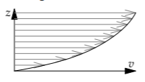
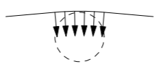
As an example, the arrows in the velocity-profile diagram show a fluid’s horizontal speed above a flat boundary—for example, the air speed above a frozen lake. Farther above the boundary, the arrows are longer, indicating that the fluid moves faster. In a high-viscosity liquid, such as honey, the viscous forces are large, and they force nearby regions move at nearly the same speed: The flow oozes.

Here is the lumped version of the velocity profile. The varying velocity has been replaced by two rectangles corresponding to two chunks of fluid. The top chunk is moving faster than the bottom chunk; because of the velocity difference, each chunk exerts a viscous force on the other.

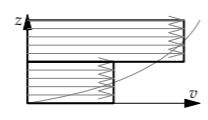
Let’s see what consequence this pair of forces has for the total energy of the chunks. To avoid cluttering the essential idea in the analysis with unit algebra, let’s give the chunks concrete velocities and masses in a simple unit system. In this unit system, both chunks will have unit mass. The top chunk will move at speed 6 and the bottom chunk at speed 4.

After a long time, how will viscosity have affected the velocities of the two slabs?

Because momentum is conserved, the final speeds sum to 10, as they do at the start. Because of the viscous force between the chunks, the top chunk slows down, and the bottom chunk speeds up. The final speeds, once viscosity has done its work, literally and figuratively, are 5 and 5.

The total kinetic energy of the two chunks starts at 26:

\[0.5 \times 1 \times (6^{2} + 4^{2}) = 26.\]

However, their final kinetic energy is only 25:

\[0.5 \times 1 \times (5^{2} + 5^{2}) = 25.\]

Simply because the velocities equalized, the kinetic energy fell! This reduction happens no matter what the initial velocities are (Problem 6.19). The energy difference turns into heat. Our simple physical model, based on lumping, is that viscosity burns up energy by equalizing velocities.

Problem 6.19: Generalizing the argument to other initial velocities

Let the initial velocities of the two chunks be \(v_{1}\) and \(v_{2}\), where \(v_{1} \neq v_{2}\). Show that the initial kinetic energy is greater than the final kinetic energy.

Problem 6.20: Shortest-time path

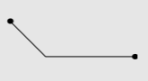
The classic problem in the calculus of variations is to find the shortest-time path for a mass sliding without friction between two points. This path is called the brachistochrone. A surprising conclusion of the full analysis is that this path need not be straight. You can make this result plausible by using shape lumping: Rather than considering all possible paths, consider only paths with one corner. Under what conditions is such a path faster than the straight path (zero corners)?

6.4.5 Mean free path

Lumping smooths out variation. In the famous words of Isaiah 40:4, the crooked shall be made straight, and the rough places plain. We’ve used this idea in Section 6.4.2 to simplify a function of time (population versus age) and in Section 6.4.4 to simplify a function of space (a velocity profile). Now we’ll combine both kinds of lumping to understand and estimate a mean free path. The mean free path is the average distance that a gas molecule travels before colliding with another molecule. As we will find in Section 7.3.1 using probabilistic reasoning, mean free paths determine important material properties, including viscosity and thermal conductivity.

Let’s first estimate the mean free path in the simplest model: a spherical molecule moving in a gas of point molecules. The sphere will have radius r and the gas molecules a number density n. After analyzing this simplified situation, we’ll replace the point molecules with more realistic spherical molecules.

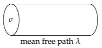
The moving molecule has a cross-sectional area \(\sigma = \pi r^{2}\), and it sweeps out a tube with the same cross-sectional area (analogous to the tube in our analysis of drag via conservation of energy in Section 3.5.1).

How far does the spherical molecule travel down the tube before it hits a point molecule?

This distance is the mean free path \(\lambda\). However, finding it is complicated because the point molecules, always in motion, keep exiting and entering the tube. Let’s simplify. First, lump in time: Freeze the motion, and pretend that the point molecules hold those positions. Then lump in space: Rather than spreading the molecules throughout the tube, place them at the far end, at a distance \(\lambda\) from the near end.

The tube, whose length is the mean free path \(\lambda\), should be just long enough so that the tube contained, before lumping, one point molecule. Then, in the lumped model with that one molecule sitting at the end of the tube, the spherical molecule will hit one molecule after traveling a distance \(\lambda\).

The number of molecules in the tube is \(n \sigma \lambda\):

\[\textrm{number} = \underbrace{\textrm{number density}}_{n} \times \underbrace{\textrm{volume}}_{\sigma \lambda} = n \sigma \lambda.\)

Therefore, \(\lambda\) is determined by the requirement that

\[n \sigma \lambda \sim 1.\]

For motion through the gas of point molecules, \(\sigma\) is \(\pi r^{2}\), so

\[\lambda \sim \frac{1}{n \pi r^{2}}.\]

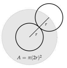
To make the model more realistic, let’s replace the point molecules with spherical molecules. For simplicity, and to model the most frequent case, these molecules will also have radius r.

How does this change affect the mean free path?

Now a collision happens if the centers of two molecules approach within a distance d = 2r, the diameter of the sphere. Thus, \(\sigma\)—called the scattering cross section—becomes \(\pi (2r)^{2}\) or \(\pi d^{2}\). The mean free path is then a factor of 4 smaller and is

\[\lambda \sim \frac{1}{n \pi d^{2}}.\]

Let’s evaluate \(\lambda\) for an air molecule traveling in air. For the diameter d, use the typical atomic diameter of 3 ångströms or 3 × 10⁻¹⁰ meters, which also works for small molecules (like air and water). To estimate the number density n, use the ideal gas law in the form that, at standard temperature and pressure, 1 mole occupies 22 liters. Therefore,

\[\frac{1}{n} = \frac{22 l}{6 \times 10^{23} \: molecules},\]

and the mean free path is

\[\lambda \sim \frac{2.2 \times 10^{-2} m^{3}}{6 \times 10^{23}} \times \frac{1}{\pi \times (3 \times 10^{-10} m)^{2}}.\]

To evaluate this expression in your head, divide the calculation into three steps—doing the most important first.

1. Units. The numerator contains cubic meters; the denominator contains square meters. Their quotient is meters to the first power—as it should be for a mean free path.

2. Powers of ten. The numerator contains −2 powers of ten. The denominator contains 3 powers of ten: 23 in Avogadro’s number and −20 in (10⁻¹⁰)². The quotient is −5 powers of ten. Along with the units, the expression so far is 10⁻⁵ meters.

3. Everything else. The remaining factors are

\[\frac{2.2}{6 \times \pi \times 3 \times 3}.\]

The 2.2/6 is roughly 10^-0.5. The three factors of 3 (one contributed by \(\pi\)) are 10^1.5. Therefore, the remaining factors contribute 10^-2.

Putting the pieces together, the mean free path becomes 10⁻⁷ meters, which is 100 nanometers—quite close to the true value of 68 nanometers.

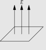
Problem 6.21: Electric field due to a uniform sheet of charge

In this problem, you investigate a physical model to estimate the electric field above a uniform sheet of charge with areal charge density \(\sigma\).

a. Explain why the electric field must be vertical.

b. At a height z above the sheet, what region of the sheet contributes significantly to this field?

c. By lumping the sheet into a point charge with the same charge as the significant region, estimate the electric field at a height z, and give the scaling exponent n in \(E \: \propto \: zn\).

Confirm your result by comparing it to the prediction from dimensional analysis (Problem 5.34).

Problem 6.22: Electric field inside a spherical shell

Another puzzling electrostatic phenomenon is that the electric field from a uniform shell of charge is zero everywhere inside the shell. At the center, the field must be zero by symmetry. However, even away from the center, the field is still zero. Explain this phenomenon using a physical model and lumping.

6.4.6 Lumping the path of light bent by gravity

Lumping, as we have seen, replaces a complex, changing process with a simpler, constant process. In the next example, we’ll use that simplification to build and analyze a physical model for the bending of starlight by the Sun. In Section 5.3.1, using dimensional analysis and educated guessing, we concluded that the bending angle is roughly \(Gm/rc^{2}\), where m is the mass of the Sun and r is the distance of closest approach (for a ray grazing the Sun, it is just the radius of the Sun). Lumping provides a physical model for this result; this model will, in Section 8.2.2.2, allow us to predict the effect of extremely strong gravitational fields.

Imagine again a beam (or photon) of light that leaves a distant star. In its journey, it grazes the surface of the Sun and reaches our eye. To estimate the deflection angle using lumping, first identify the changing process—the source of the complexity. Here, the light beam deflects from its original, straight path and the gravitational force from the Sun changes in magnitude and direction as the photon travels. Therefore, calculating the deflection angle requires setting up and evaluating an integral—and carefully checking its trigonometric factors, such as the cosines and secants.

The antidote to complicated integrals is lumping. The lumping approximation simply pretends that the beam bends only near the Sun. In this approximation, only near the Sun does gravity operate. We further assume that, while the photon is near the Sun, its downward acceleration (the acceleration perpendicular to the path) is constant, rather than varying rapidly with position.

The problem then simplifies to estimating the deflection while the beam is near the Sun. As a further lumping approximation, let’s define “near” to mean “within r on either side of the location of closest approach.” The justification is dimensional: The only length in the problem is the distance of closest approach, which is r; therefore, “near” and “far” are defined relative to the characteristic distance r.

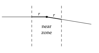
The geometry is simplest at the point of closest approach. Therefore, let’s make the further lumping approximation that, although the light beam tracks how much downward deflection should happen, the total deflection happens only at the point of closest approach.

This lumped path, instead of changing direction smoothly, has a kink (a corner) at the point of closest approach.

The deflection angle, in the small-angle approximation, is the ratio of velocity components:

\[\theta \approx \frac{v_{\downarrow}}{c}, \]

where c is the speed of light, which is the forward velocity, and \(v_{\downarrow}\) is the accumulated downward velocity. This downward velocity comes from the downward acceleration due to the Sun’s gravity.

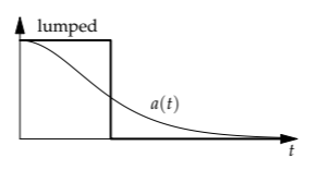
In the exact analysis, the downward acceleration varies along the path. As a function of time, it looks like a bell curve centered at the point of closest approach (labeled as t = 0, for symmetry). The downward velocity is the integral of (the area under) the entire \(a_{downarrow}(t)\) curve.

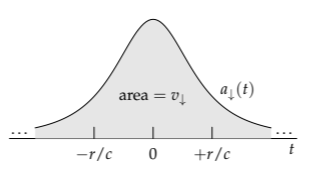
Our lumping analysis replaces the entire area by a rectangle centered around the peak. This rectangle has height \(Gm/r^{2}\): the characteristic (and peak) downward acceleration. It has width comparable to \(r/c\): the time that the beam spends near the Sun. Therefore, its area, which is the lumping approximation to \(v_{\downarrow}\), is roughly \(Gm/rc\):

\[\underbrace{v_{\downarrow}}_{Gm/rc} \sim \underbrace{\textrm{characteristic downward acceleration}}_{Gm/r^{2}} \times \underbrace{\textrm{deflection time.}}_{\sim r/c}\]

The deflection angle is therefore comparable to \(Gm/rc^{2}\):

\[\theta \sim \overbrace{\frac{Gm/rc}{c}}^{v_{\downarrow}} = \frac{Gm}{rc^{2}}.\]

The lumping argument explains, with a physical model, the deflection angle that we predicted using dimensional analysis and educated guessing (Section 5.3.1). Lumping once again complements dimensional analysis.

Problem 6.23: Sketching the actual and lumped deflection angle

On axes for cumulative deflection \(\theta\) versus distance along the beam, sketch (a) the actual curve, (b) the lumped curve, assuming that the deflection happens only while the beam is near the Sun, and (c) the lumped curve, assuming, as in the text, that the deflection happens only at the point of closest approach.

6.4.7 All-or-nothing reasoning: Solid mechanics by lumping

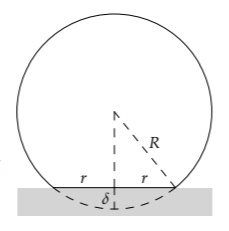
For estimating the bending of light, the heart of the lumping analysis was all-or-nothing reasoning: replacing the complex, varying downward acceleration with a simpler curve that was either zero or a nonzero constant. To practice this idea, we’ll apply it to an example from solid mechanics, also a subject fraught with differential equations. In particular, we’ll estimate the contact radius of a solid ball resting on the ground.

We know a bit about the contact radius: In Problem 5.50, you used dimensional analysis to find that the contact radius r is given by

\[\frac{r}{R} = f(\frac{\rho g R}{Y}),\]

where R is the ball’s radius, \(\rho\) is its density, Y is its Young’s modulus, and f is a dimensionless function. The function f is not determined by dimensional analysis, which is purely mathematical reasoning. Finding f requires a physical model; the easiest way to make and analyze such a model is by making lumping approximations.

Physically, the ground compresses the tip of the ball by a small distance \(\delta\), making a flat circle of radius r in contact with the ground. The ball fights back, trying to restore its natural, spherical shape. When the ball rests on the table, the restoring force equals its weight. This constraint will give us enough information to find the dimensionless function f.

The restoring force comes from the stress (or pressure) over the contact surface. To estimate this stress, let’s make the lumping approximation that it is constant over the contact surface and equal to a typical or characteristic stress. This approximation is analogous to replacing the varying population curve with a constant value (and making a rectangle). With that approximation, the restoring force is

\[\textrm{force} \sim \textrm{typical stress}\times \textrm{contact area}.\]

We can estimate the stress based on the strain (the fractional compression). The stress and strain are related by the Young’s modulus Y:

\[\textrm{typical stress} \sim Y \times \textrm{typical strain}.\]

The strain, like the stress, varies throughout the ball. In the lumping or all-or-nothing approximation, the strain becomes a characteristic or typical strain in a region around the contact surface, and zero outside this region. The typical strain is a fractional length change:

\[\textrm{strain} = \frac{\textrm{length change}}{\textrm{length}}.\]

The numerator is \(\delta\): the amount by which the tip of the ball is compressed. The denominator is the size of the mysterious compressed region.

How large is the compressed region?

Because the ball’s radius or diameter changes, the compressed region might be the whole ball. This tempting reasoning turns out to be incorrect. To see why, imagine an extreme case: compressing a huge, 10-meter cube of rubber (rubber, because one can imagine compressing it). By pressing your finger onto the center of one face, you’ll indent the face by, say, 1 millimeter over an area of 1 square centimeter. In the notation that we use for the ball, \(\delta\) ~ 1 millimeter, r ~ 1 centimeter, and R ~ 10 meters.

The strained region is not the whole cube, nor any significant fraction of it! Rather, its radius is comparable to the radius of the contact region—a fingertip (r ∼ 1 centimeter). From this thought experiment, we learn that when the object is large enough (R ≫ r), the strained volume is related not to the size of the object, but rather to the size of contact region (r).

Therefore, in the estimate for the typical strain, the length in the denominator is r. The typical strain \(\epsilon\) is then \(\delta/r\).

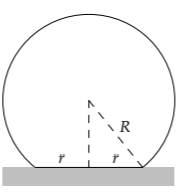
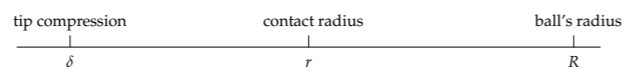
Because the compression \(\delta\), in contrast to the contact radius r and the ball’s radius R, is not easily visible, let’s rewrite \(\delta\) in terms of r and R. Amazingly, they are related by a geometric mean, because their geometry reproduces the geometry of the horizon distance (Section 2.3). The compression \(\delta\) is analogous to one’s height above sea level. The contact radius r is analogous to the horizon distance. And the ball’s radius R is analogous to the Earth’s radius.

Just as the horizon distance is roughly the geometric mean of the two surrounding lengths, so should the contact radius be roughly the geometric mean of the compression length and the ball’s radius. On a logarithmic scale, r is roughly halfway between \(\delta\) and R. (Like the horizon distance, r is actually halfway between \*\delta\) and the diameter 2R. However, the factor of 2 does not matter to this lumping analysis.)

Therefore, \(\delta/r\), which is the typical strain, is also roughly \(r/R\). The restoring force is therefore comparable to \(Yr^{3}/R\):

\[\underbrace{\textrm{restoring force}}_{Yr^{3}/R} \sim \overbrace{Y \times \underbrace{\textrm{typical strain}}_{r/R}}^{\textrm{typical stress}} \times \underbrace{\textrm{contact area}}_{r^{2}}.\]

This force balances the weight, which is comparable to \(\rho g R^{3}\):

\[\frac{Y r^{3}}{R} \sim \rho g R^{3}.\]

Therefore, in dimensionless form, the contact radius is given by

\[\frac{r}{R} \sim (\frac{\rho g R}{Y})^{1/3},\]

and the dimensionless function f in

\[\frac{r}{R} = f(\frac{\rho gR}{Y})\]

is a cube root (multiplied by a dimensionless constant).

How large is the contact radius \(r\) in practice?

Let’s plug in numbers for a superball (a small, highly elastic rubber ball) resting on the ground. The density of rubber is roughly the density of water. A superball is small—say, R ∼ 1 centimeter. Its elastic modulus is roughly Y ∼ 3 × 10⁷ pascals. (This elastic modulus is a factor of 300 smaller than oak’s and almost a factor of 10⁴ smaller than steel’s.) Then

\[\frac{r}{R} \sim(\frac{\overbrace{10^{3} kg/m^{3}}^{\rho} \times \overbrace{10 m s^{-2}}^{g} \times \overbrace {10^{-2}m}^{R}}{\underbrace{3 \times 10^{7}Pa}_{Y}})^{1/3}.\]

The quotient inside the parentheses is 10^−5.5. Its cube root is roughly 10⁻², so r/R is roughly 10⁻², and r is roughly 0.1 millimeters (a sheet of paper).

From this example, we see how lumping builds on dimensional analysis. Dimensional analysis gave the form of the relation between \(r/R\) and \(\rho g R/Y\). Lumping provided a physical model that specified the particular form.

Problem 6.24: Compression of the tip

For the superball, estimate \(\delta\), the compression of its tip when it is resting on the ground

Problem 6.25: Contact radius of a marble

Estimate the contact radius of a small glass marble sitting on a (very) hard table

Problem 6.26: Energy argument

The potential-energy density due to deforming a solid is comparable to \(Y \epsilon ^{2}\). Using this relation, find a second explanation for why \(r/R\) is comparable to \(\rho g R/Y)^{1/3}\).

Problem 6.27: Mountain heights

On Earth, the tallest mountain (Everest) is 9 kilometers high. On Mars, the tallest mountain (Olympus) is 27 kilometers high. Make a lumped model of a mountain to explain the factor-of-3 difference. If the same reasoning applied to the Moon, how high would its tallest mountain be? Why is it so much shorter?

Problem 6.28: Asteroid shapes

The tallest mountain on Earth is much smaller than the Earth. Using the mountain-height data of Problem 6.27, estimate the maximum radius of a planetary body made of rock (like the Earth or Mars) that has mountains comparable in size to the body. What consequence does this size have for the shapes of asteroids?

Problem 6.29: Contact time

Imagine a ball dropped from a height, hitting a hard table with impact speed \(v\). Find the scaling exponent \(\beta\) in

\[\frac{\tau c_{s}}{R} \sim (\frac{v}{c_{s}})^{\beta},\]

where \(\tau\) is the contact time and c_s is the speed of sound in the ball. Then write \(\tau\) in the form \(\tau \sim R/v_{effective}\), where v_effective is a weighted geometric mean of the impact speed \(v\) and the sound speed c_s.

Problem 6.30: Contact force

For a small steel ball bouncing from a steel table with impact speed 1 meter per second (Problem 6.29), how large is the contact force compared to the ball’s weight?