1.7: Hencky Relations
- Page ID
- 7784
\( \newcommand{\vecs}[1]{\overset { \scriptstyle \rightharpoonup} {\mathbf{#1}} } \)
\( \newcommand{\vecd}[1]{\overset{-\!-\!\rightharpoonup}{\vphantom{a}\smash {#1}}} \)
\( \newcommand{\dsum}{\displaystyle\sum\limits} \)
\( \newcommand{\dint}{\displaystyle\int\limits} \)
\( \newcommand{\dlim}{\displaystyle\lim\limits} \)
\( \newcommand{\id}{\mathrm{id}}\) \( \newcommand{\Span}{\mathrm{span}}\)
( \newcommand{\kernel}{\mathrm{null}\,}\) \( \newcommand{\range}{\mathrm{range}\,}\)
\( \newcommand{\RealPart}{\mathrm{Re}}\) \( \newcommand{\ImaginaryPart}{\mathrm{Im}}\)
\( \newcommand{\Argument}{\mathrm{Arg}}\) \( \newcommand{\norm}[1]{\| #1 \|}\)
\( \newcommand{\inner}[2]{\langle #1, #2 \rangle}\)
\( \newcommand{\Span}{\mathrm{span}}\)
\( \newcommand{\id}{\mathrm{id}}\)
\( \newcommand{\Span}{\mathrm{span}}\)
\( \newcommand{\kernel}{\mathrm{null}\,}\)
\( \newcommand{\range}{\mathrm{range}\,}\)
\( \newcommand{\RealPart}{\mathrm{Re}}\)
\( \newcommand{\ImaginaryPart}{\mathrm{Im}}\)
\( \newcommand{\Argument}{\mathrm{Arg}}\)
\( \newcommand{\norm}[1]{\| #1 \|}\)
\( \newcommand{\inner}[2]{\langle #1, #2 \rangle}\)
\( \newcommand{\Span}{\mathrm{span}}\) \( \newcommand{\AA}{\unicode[.8,0]{x212B}}\)
\( \newcommand{\vectorA}[1]{\vec{#1}} % arrow\)
\( \newcommand{\vectorAt}[1]{\vec{\text{#1}}} % arrow\)
\( \newcommand{\vectorB}[1]{\overset { \scriptstyle \rightharpoonup} {\mathbf{#1}} } \)
\( \newcommand{\vectorC}[1]{\textbf{#1}} \)
\( \newcommand{\vectorD}[1]{\overrightarrow{#1}} \)
\( \newcommand{\vectorDt}[1]{\overrightarrow{\text{#1}}} \)
\( \newcommand{\vectE}[1]{\overset{-\!-\!\rightharpoonup}{\vphantom{a}\smash{\mathbf {#1}}}} \)
\( \newcommand{\vecs}[1]{\overset { \scriptstyle \rightharpoonup} {\mathbf{#1}} } \)
\(\newcommand{\longvect}{\overrightarrow}\)
\( \newcommand{\vecd}[1]{\overset{-\!-\!\rightharpoonup}{\vphantom{a}\smash {#1}}} \)
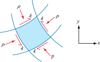
\(\newcommand{\avec}{\mathbf a}\) \(\newcommand{\bvec}{\mathbf b}\) \(\newcommand{\cvec}{\mathbf c}\) \(\newcommand{\dvec}{\mathbf d}\) \(\newcommand{\dtil}{\widetilde{\mathbf d}}\) \(\newcommand{\evec}{\mathbf e}\) \(\newcommand{\fvec}{\mathbf f}\) \(\newcommand{\nvec}{\mathbf n}\) \(\newcommand{\pvec}{\mathbf p}\) \(\newcommand{\qvec}{\mathbf q}\) \(\newcommand{\svec}{\mathbf s}\) \(\newcommand{\tvec}{\mathbf t}\) \(\newcommand{\uvec}{\mathbf u}\) \(\newcommand{\vvec}{\mathbf v}\) \(\newcommand{\wvec}{\mathbf w}\) \(\newcommand{\xvec}{\mathbf x}\) \(\newcommand{\yvec}{\mathbf y}\) \(\newcommand{\zvec}{\mathbf z}\) \(\newcommand{\rvec}{\mathbf r}\) \(\newcommand{\mvec}{\mathbf m}\) \(\newcommand{\zerovec}{\mathbf 0}\) \(\newcommand{\onevec}{\mathbf 1}\) \(\newcommand{\real}{\mathbb R}\) \(\newcommand{\twovec}[2]{\left[\begin{array}{r}#1 \\ #2 \end{array}\right]}\) \(\newcommand{\ctwovec}[2]{\left[\begin{array}{c}#1 \\ #2 \end{array}\right]}\) \(\newcommand{\threevec}[3]{\left[\begin{array}{r}#1 \\ #2 \\ #3 \end{array}\right]}\) \(\newcommand{\cthreevec}[3]{\left[\begin{array}{c}#1 \\ #2 \\ #3 \end{array}\right]}\) \(\newcommand{\fourvec}[4]{\left[\begin{array}{r}#1 \\ #2 \\ #3 \\ #4 \end{array}\right]}\) \(\newcommand{\cfourvec}[4]{\left[\begin{array}{c}#1 \\ #2 \\ #3 \\ #4 \end{array}\right]}\) \(\newcommand{\fivevec}[5]{\left[\begin{array}{r}#1 \\ #2 \\ #3 \\ #4 \\ #5 \\ \end{array}\right]}\) \(\newcommand{\cfivevec}[5]{\left[\begin{array}{c}#1 \\ #2 \\ #3 \\ #4 \\ #5 \\ \end{array}\right]}\) \(\newcommand{\mattwo}[4]{\left[\begin{array}{rr}#1 \amp #2 \\ #3 \amp #4 \\ \end{array}\right]}\) \(\newcommand{\laspan}[1]{\text{Span}\{#1\}}\) \(\newcommand{\bcal}{\cal B}\) \(\newcommand{\ccal}{\cal C}\) \(\newcommand{\scal}{\cal S}\) \(\newcommand{\wcal}{\cal W}\) \(\newcommand{\ecal}{\cal E}\) \(\newcommand{\coords}[2]{\left\{#1\right\}_{#2}}\) \(\newcommand{\gray}[1]{\color{gray}{#1}}\) \(\newcommand{\lgray}[1]{\color{lightgray}{#1}}\) \(\newcommand{\rank}{\operatorname{rank}}\) \(\newcommand{\row}{\text{Row}}\) \(\newcommand{\col}{\text{Col}}\) \(\renewcommand{\row}{\text{Row}}\) \(\newcommand{\nul}{\text{Nul}}\) \(\newcommand{\var}{\text{Var}}\) \(\newcommand{\corr}{\text{corr}}\) \(\newcommand{\len}[1]{\left|#1\right|}\) \(\newcommand{\bbar}{\overline{\bvec}}\) \(\newcommand{\bhat}{\widehat{\bvec}}\) \(\newcommand{\bperp}{\bvec^\perp}\) \(\newcommand{\xhat}{\widehat{\xvec}}\) \(\newcommand{\vhat}{\widehat{\vvec}}\) \(\newcommand{\uhat}{\widehat{\uvec}}\) \(\newcommand{\what}{\widehat{\wvec}}\) \(\newcommand{\Sighat}{\widehat{\Sigma}}\) \(\newcommand{\lt}{<}\) \(\newcommand{\gt}{>}\) \(\newcommand{\amp}{&}\) \(\definecolor{fillinmathshade}{gray}{0.9}\)Unless \( \tau_{x y}=\pm k_{i} \), where \( k \) is the shear yield stress, the \(x\)- and \(y\)-directions (or axes) will not correspond to the directions of the \(\alpha - \) and \( \beta - \) slip lines, which are themselves at ± 45° to the directions of principal stresses acting on the element. In general, we need to examine the stresses on a small curvilinear element in the \(x\) - \( y \) plane upon which a shear stress and a hydrostatic stress are acting, and where the principal stresses are \( – p – k \) and \(– p + k \) for a situation where there is plane strain compression, such as in forging or indentation in which \( k \) is a constant but \( p \) can vary from point to point:

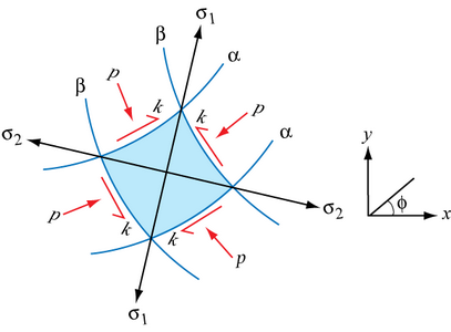
We can then identify on this diagram the directions of principal stress \( \sigma_1 \) and \( \sigma_2 \) (remembering that \( \sigma_1 > \sigma_2 \), and which of the lines are \(\alpha\)-lines and which are \(\beta\)-lines. We can also specify the angle \( \varphi \) of the \(\alpha\)-lines with respect to the \(x\)-axis:

Suppose that the \(\alpha\)-slip line passing through the element makes an angle \( \varphi \) with respect to reference \(x\)- and \(y\)-axes, as in the above diagram. The \(\beta\)-slip line must then make an angle of 90° \(+ \varphi \) with respect to the x-axis, so that an anticlockwise rotation from the \(\alpha\)-slip line to the \(\beta\)-slip line crosses the direction of maximum principal stress, \( \sigma_1 \).
The direction parallel to the principal stress \( \sigma_1 \) makes an angle of 45° \( +\varphi \) with respect to the \(x\)-axis and the direction parallel to the principal stress \( \sigma_2 \) makes an angle of \( 135^{\circ}+\varphi^{\circ} 45^{\circ}-\varphi \) with respect to the \(x\)-axis.
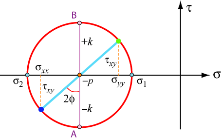
On a Mohr’s circle, this all looks like:

where A and B represent the stress states along the \(\alpha\)- and \(\beta\)-lines respectively.
Hence, from the above,
\[ \sigma_{x x}=-p-k \sin 2 \varphi \]
\[ \sigma_{y y}=-p+k \sin 2 \varphi \]
\[ \tau_{x y}=k \cos 2 \varphi \]
while the tensile stress in the \(z\)-direction in plain strain plastic yielding is simply:
\[ \frac{1}{2}\left(\sigma_{x x}+\sigma_{y y}\right)=-p \]
Substituting these expressions into the equilibrium equations
\[\frac{\partial \sigma_{x x}}{\partial x}+\frac{\partial \tau_{x y}}{\partial y}=0 \]
\[ \frac{\partial \tau_{x y}}{\partial x}+\frac{\partial \sigma_{y y}}{\partial y}=0 \]
and recognizing that \(k\) is a constant independent of \(x\) and \(y\), we obtain two equations for \(p\) and \(\varphi\) as a function of \(x\) and \(y\):
\[ -\frac{\partial p}{\partial x}-2 k \cos 2 \varphi \frac{\partial \varphi}{\partial x}-2 k \sin 2 \varphi \frac{\partial \varphi}{\partial y}=0 \]
\[ -2 k \sin 2 \varphi \frac{\partial \varphi}{\partial x}-\frac{\partial p}{\partial y}+2 k \cos 2 \varphi \frac{\partial \varphi}{\partial y}=0 \]
For \(\varphi=0^{\circ}\), in which case the \(\alpha\) and \(\beta\) lines coincide with the external \(x\)- and \(y\)-axes respectively at a particular position, these equations become
\[ \frac{\partial}{\partial x}(p+2 k \varphi)=0 \]
\[ \frac{\partial}{\partial y}(p-2 k \varphi)=0 \]
Integrating these equations we find
\[ p+2 k \varphi=f_{1}(y)+C_{1} \label{eq:1}\]
\[ p-2 k \varphi=f_{2}(x)+C_{2} \label{eq:2}\]
as the most general form of the solutions of these two partial differential equations. However, we know that when \(\varphi\) is exactly zero, \(p\) must have the same value in both Equations \(\ref{eq:1}\) and Eq. \(\ref{eq:2}\). Hence it follows that \(f_{1}(x)=f_{2}(y)=0\).
In general for points in a slip-line field we have therefore proved that the Hencky relations have to be satisfied:
Hencky relations
The hydrostatic pressure \(p\) varies linearly with the angle \(\varphi\) turned by a slip line.
- \( p+2 k \varphi\) is constant along an \(\alpha\) line
- \( p-2 k \varphi\) is constant along a \(\beta\) line
where the angle φ is in radians.


