14.3: Representing Texture

Pole figures

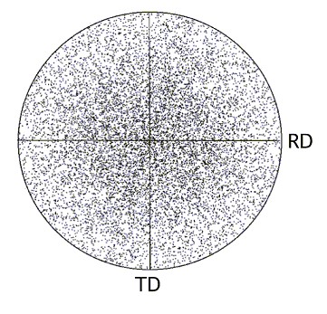
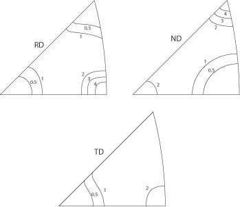
A pole figure is simply a stereogram with its axes defined by an external frame of reference with particular hkl poles plotted onto it from all of the crystallites in the polycrystal. Typically, the external frame is defined by the normal direction, the rolling direction, and the transverse direction in a sheet (ND, RD and TD respectively. Occasionally, CD meaning cross direction is used instead of TD.)

The animation below shows the relationship between the orientation of the crystal and the stereographic projection obtained for the <100> poles. Drag an atom in the green sphere to reorientate the unit cell of the grain under consideration. This will alter the projections of the [100], [010] and [001] directions on the stereogram inside the rectangle. Press 'Add grain' to add the [100], [010] and [001] directions of another grain, up to a maximum of four additional grains. Try altering their orientations so that all five are similar and then different, and notice how the positions of the poles change.

A pole figure for a polycrystalline aggregate, which shows completely random orientation, does not necessarily appear as might naively be expected. Angular distortions inherent in the stereographic projection result in the accumulation of points close to the centre of the pole figure as shown in the image below.

If the material shows a degree of texture, the resultant pole figure will show the accumulation of poles about specific directions.

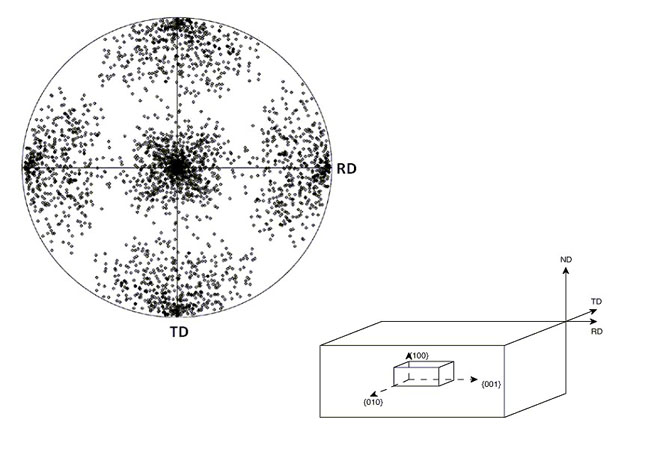
A 100 pole figure showing “cube” texture – the {100} poles of the crystallites are oriented so that they are aligned with the axes defined by the rolling, transverse, and normal directions.

A single crystal can be plotted on the pole figure and there is no ambiguity regarding its orientation. However, as more crystallite poles are plotted onto the pole figure, the specific orientation of a particular crystallite can no longer be defined.

For a large number of grains in a polycrystal, poles may overlap on the pole figure, so that the true orientation density is not clearly represented. In this case, contours tend to be used instead. Regions of high pole density have a high number of contours, while regions with low pole density have a few, greatly spaced contours.

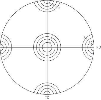
100 pole figure showing “cube” texture and pole density represented using contours rather than discrete points.

Inverse pole figures

Instead of plotting crystal orientations with respect to an external frame of reference, inverse pole figures can be produced which show the rolling, transverse, and normal directions (RD, TD and ND respectively) with respect to the crystallographic axes. Typically, these are plotted on a standard stereographic triangle as shown below

Crystal Orientation Distribution Function (CODF)

As previously mentioned, pole figures do not give information about the orientation of a particular crystal relative to another. More information can be gathered from a CODF. CODFs are constructed by combining the data from several pole figures. This requires intensive use of mathematics. More details can be found in the references listed in the Going further section.

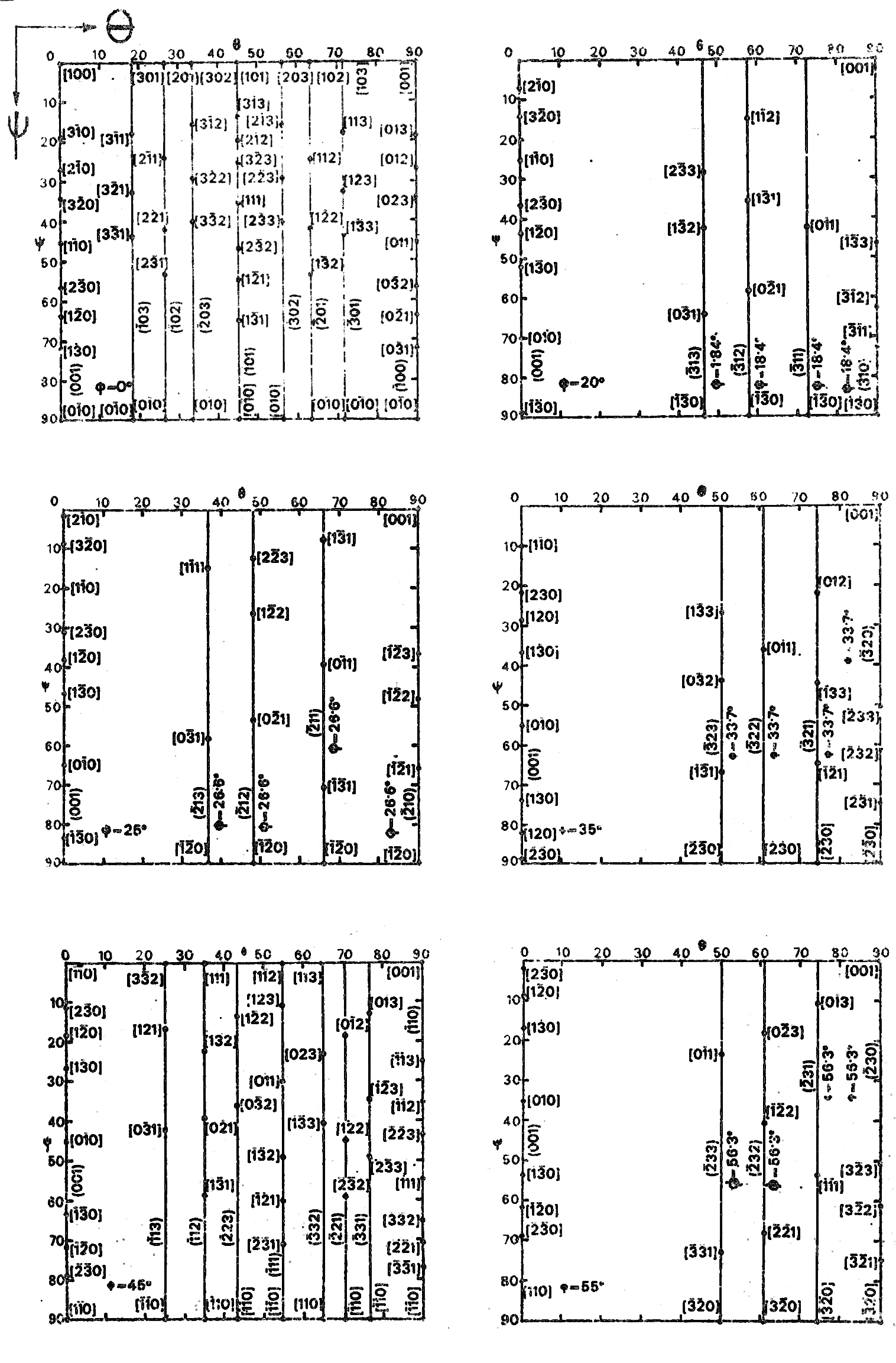
CODFs describe the orientation of each crystal relative to three Euler angles (φ,ψ, and θ). The Euler angles define the difference in orientation between the crystal axes and the deformation axes (i.e. the RD, the ND and the TD).

Note: This animation requires Adobe Flash Player 8 and later, which can be downloaded here.

One convention for Euler angles (and the convention described here) is known as the Roe convention. An alternative convention can be used where the θ-rotation occurs about the x1 direction; this is known as the Bunge convention. These two conventions are related by:

ψ_Roe = ψ_1,Bunge – π/2
θ_Roe = φ_Bunge
φ_Roe = ψ_{2, Bunge} + π/2

A single crystal is completely described by a point in a cube with axes of φ, ψ and θ. This cube is referred to as Euler space and is often shown as a series of cross-sections.

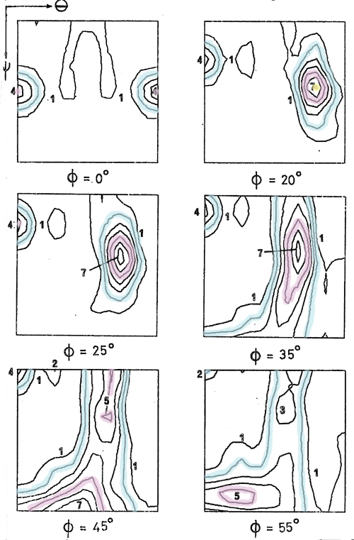
These sections of a CODF are for a steel sheet cold-rolled to an 80% reduction in thickness. Any values of φ between 0° and 90° can be used to produce the sections. In the image above, the values of φ that have been chosen are: 0°, 20°, 25°, 35°, 45°, and 55°. The contours of the sections make up part of a three-dimensional surface in Euler space as seen in the following animation. The highlighted contours on the sections correspond to the similarly coloured surface in the 3D plot below. The area of highest density and hence strongest texture is bound by the yellow surface centred around φ = 26.6°, ψ = 39.2°, and θ = 65.9°. The original figure can be found in D.J. Goodwill Ph.D. thesis, University of Cambridge (1972) – The relationship between texture and properties of steel sheets.

Note: This animation requires Adobe Flash Player 8 and later, which can be downloaded here.

Texture diagrams such as those produced by Davies, Goodwill, and Kallend (1971) (See Going further) can be used to identify the texture present. In this case it is (211)[011]. (211) describes a plane which is orientated parallel to the plane of the sheet, while [011] is a direction parallel to the rolling direction.