23.6: J-Shaped Curves
- Page ID
- 32710
\( \newcommand{\vecs}[1]{\overset { \scriptstyle \rightharpoonup} {\mathbf{#1}} } \)
\( \newcommand{\vecd}[1]{\overset{-\!-\!\rightharpoonup}{\vphantom{a}\smash {#1}}} \)
\( \newcommand{\dsum}{\displaystyle\sum\limits} \)
\( \newcommand{\dint}{\displaystyle\int\limits} \)
\( \newcommand{\dlim}{\displaystyle\lim\limits} \)
\( \newcommand{\id}{\mathrm{id}}\) \( \newcommand{\Span}{\mathrm{span}}\)
( \newcommand{\kernel}{\mathrm{null}\,}\) \( \newcommand{\range}{\mathrm{range}\,}\)
\( \newcommand{\RealPart}{\mathrm{Re}}\) \( \newcommand{\ImaginaryPart}{\mathrm{Im}}\)
\( \newcommand{\Argument}{\mathrm{Arg}}\) \( \newcommand{\norm}[1]{\| #1 \|}\)
\( \newcommand{\inner}[2]{\langle #1, #2 \rangle}\)
\( \newcommand{\Span}{\mathrm{span}}\)
\( \newcommand{\id}{\mathrm{id}}\)
\( \newcommand{\Span}{\mathrm{span}}\)
\( \newcommand{\kernel}{\mathrm{null}\,}\)
\( \newcommand{\range}{\mathrm{range}\,}\)
\( \newcommand{\RealPart}{\mathrm{Re}}\)
\( \newcommand{\ImaginaryPart}{\mathrm{Im}}\)
\( \newcommand{\Argument}{\mathrm{Arg}}\)
\( \newcommand{\norm}[1]{\| #1 \|}\)
\( \newcommand{\inner}[2]{\langle #1, #2 \rangle}\)
\( \newcommand{\Span}{\mathrm{span}}\) \( \newcommand{\AA}{\unicode[.8,0]{x212B}}\)
\( \newcommand{\vectorA}[1]{\vec{#1}} % arrow\)
\( \newcommand{\vectorAt}[1]{\vec{\text{#1}}} % arrow\)
\( \newcommand{\vectorB}[1]{\overset { \scriptstyle \rightharpoonup} {\mathbf{#1}} } \)
\( \newcommand{\vectorC}[1]{\textbf{#1}} \)
\( \newcommand{\vectorD}[1]{\overrightarrow{#1}} \)
\( \newcommand{\vectorDt}[1]{\overrightarrow{\text{#1}}} \)
\( \newcommand{\vectE}[1]{\overset{-\!-\!\rightharpoonup}{\vphantom{a}\smash{\mathbf {#1}}}} \)
\( \newcommand{\vecs}[1]{\overset { \scriptstyle \rightharpoonup} {\mathbf{#1}} } \)
\(\newcommand{\longvect}{\overrightarrow}\)
\( \newcommand{\vecd}[1]{\overset{-\!-\!\rightharpoonup}{\vphantom{a}\smash {#1}}} \)
\(\newcommand{\avec}{\mathbf a}\) \(\newcommand{\bvec}{\mathbf b}\) \(\newcommand{\cvec}{\mathbf c}\) \(\newcommand{\dvec}{\mathbf d}\) \(\newcommand{\dtil}{\widetilde{\mathbf d}}\) \(\newcommand{\evec}{\mathbf e}\) \(\newcommand{\fvec}{\mathbf f}\) \(\newcommand{\nvec}{\mathbf n}\) \(\newcommand{\pvec}{\mathbf p}\) \(\newcommand{\qvec}{\mathbf q}\) \(\newcommand{\svec}{\mathbf s}\) \(\newcommand{\tvec}{\mathbf t}\) \(\newcommand{\uvec}{\mathbf u}\) \(\newcommand{\vvec}{\mathbf v}\) \(\newcommand{\wvec}{\mathbf w}\) \(\newcommand{\xvec}{\mathbf x}\) \(\newcommand{\yvec}{\mathbf y}\) \(\newcommand{\zvec}{\mathbf z}\) \(\newcommand{\rvec}{\mathbf r}\) \(\newcommand{\mvec}{\mathbf m}\) \(\newcommand{\zerovec}{\mathbf 0}\) \(\newcommand{\onevec}{\mathbf 1}\) \(\newcommand{\real}{\mathbb R}\) \(\newcommand{\twovec}[2]{\left[\begin{array}{r}#1 \\ #2 \end{array}\right]}\) \(\newcommand{\ctwovec}[2]{\left[\begin{array}{c}#1 \\ #2 \end{array}\right]}\) \(\newcommand{\threevec}[3]{\left[\begin{array}{r}#1 \\ #2 \\ #3 \end{array}\right]}\) \(\newcommand{\cthreevec}[3]{\left[\begin{array}{c}#1 \\ #2 \\ #3 \end{array}\right]}\) \(\newcommand{\fourvec}[4]{\left[\begin{array}{r}#1 \\ #2 \\ #3 \\ #4 \end{array}\right]}\) \(\newcommand{\cfourvec}[4]{\left[\begin{array}{c}#1 \\ #2 \\ #3 \\ #4 \end{array}\right]}\) \(\newcommand{\fivevec}[5]{\left[\begin{array}{r}#1 \\ #2 \\ #3 \\ #4 \\ #5 \\ \end{array}\right]}\) \(\newcommand{\cfivevec}[5]{\left[\begin{array}{c}#1 \\ #2 \\ #3 \\ #4 \\ #5 \\ \end{array}\right]}\) \(\newcommand{\mattwo}[4]{\left[\begin{array}{rr}#1 \amp #2 \\ #3 \amp #4 \\ \end{array}\right]}\) \(\newcommand{\laspan}[1]{\text{Span}\{#1\}}\) \(\newcommand{\bcal}{\cal B}\) \(\newcommand{\ccal}{\cal C}\) \(\newcommand{\scal}{\cal S}\) \(\newcommand{\wcal}{\cal W}\) \(\newcommand{\ecal}{\cal E}\) \(\newcommand{\coords}[2]{\left\{#1\right\}_{#2}}\) \(\newcommand{\gray}[1]{\color{gray}{#1}}\) \(\newcommand{\lgray}[1]{\color{lightgray}{#1}}\) \(\newcommand{\rank}{\operatorname{rank}}\) \(\newcommand{\row}{\text{Row}}\) \(\newcommand{\col}{\text{Col}}\) \(\renewcommand{\row}{\text{Row}}\) \(\newcommand{\nul}{\text{Nul}}\) \(\newcommand{\var}{\text{Var}}\) \(\newcommand{\corr}{\text{corr}}\) \(\newcommand{\len}[1]{\left|#1\right|}\) \(\newcommand{\bbar}{\overline{\bvec}}\) \(\newcommand{\bhat}{\widehat{\bvec}}\) \(\newcommand{\bperp}{\bvec^\perp}\) \(\newcommand{\xhat}{\widehat{\xvec}}\) \(\newcommand{\vhat}{\widehat{\vvec}}\) \(\newcommand{\uhat}{\widehat{\uvec}}\) \(\newcommand{\what}{\widehat{\wvec}}\) \(\newcommand{\Sighat}{\widehat{\Sigma}}\) \(\newcommand{\lt}{<}\) \(\newcommand{\gt}{>}\) \(\newcommand{\amp}{&}\) \(\definecolor{fillinmathshade}{gray}{0.9}\)Descriptions of J-Shaped Curves
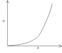
Many biomaterials exhibit the following type of stress-strain curve, which is known as a J-shaped curve:

A J-shaped stress-strain curve
The curve shows that initially, small increases in stress give large extensions, however, at larger extensions the material becomes stiffer, and more difficult to extend. Mammalian skin and flesh are two of the many biomaterials that exhibit a J-shaped curve. If you pinch your earlobe and try to pull it downwards, you will see that initially it is quite easy to stretch the earlobe, but that at larger extensions it becomes more difficult to stretch.
Loading and unloading occurs along the same curve, i.e. the loading is completely reversible and elastic. This ensures that all the energy used in extending the system is returned once the load is removed. It is clearly important that there should not be too much energy absorption in arterial walls. The elastic properties of arterial wall are important not only to protect against aneurysms, but to smooth out variations in blood pressure and blood flow rate.
Advantages of J-shaped curves for biomaterials
J-shaped stress-strain curves cause biological membranes to be extremely tough, even though the fracture energy for many materials is not particularly high (around 10 kJ m-2). This toughness arises for the following reasons:
- The lower part of the J-shaped curve gives very large extension for low applied stress, so the shear modulus in this region is very low and so there is no mechanism whereby the released strain energy on fracture can be transmitted to the fracture zone.
- The material gets stiffer as the failure point approaches ensuring that very large extensions require large stresses, so that extensions which are likely to cause harm occur infrequently.
- Since the J-shaped curve is concave, the area under the curve up to a given extension is far lower than that for the equivalent Hookean curve meaning that the energy released in the fracture of a material with a J-shaped stress-strain curve is far lower than the energy released when an equivalent Hookean material fails. Since the release of energy drives crack propagation, a material that releases less energy on fracture is tougher.
- The J-shaped stress-strain curve does not lead to the elastic instabilities such as aneurysms which arise with S-shaped curves. Hence J-shaped curves are favoured for arteries.
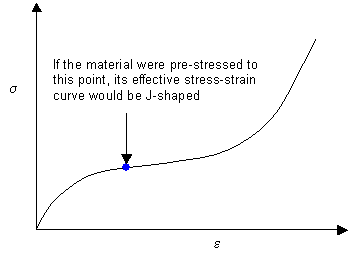
A J-shaped curve can be compared to an S-shaped curve in which the material has been pre-stressed, causing the effective origin of the graph to be further along the curve. This is shown below. Arteries are naturally pre-stressed as even the minimum blood pressure must be sufficiently positive to raise blood to the highest point of the body.

How Does the J-Shaped Curve Arise?
The J-shaped curve can arise at a number of different structural levels. For a J-shaped curve to arise, there must simply be the progressive recruitment of strain-resistant components. This can occur by the progressive alignment of polymer chains with the stress, and indeed, the stress-strain curve of a rubber is (at higher extensions) J-shaped. Many biomaterials are pre-stressed rubbery materials (i.e. in their neutral position they are still under tension). These rubbery materials, by virtue of being pre-stressed, show only J-shaped behaviour. A similar effect occurs in materials that contain fibres in a soft matrix. Initially the stress acts only against the soft matrix, but with time the fibres align in the direction of the stress and so further pulling works against the stiffer fibres. This effect is used in arterial walls, where the collagen fibres act as the stiffer fibres. (More information on the structure of arterial walls.)
Examples of Materials With J-Shaped Stress-Strain Curves
Textile materials provide some non-biological examples of materials with J-shaped stress-strain curves. Knitted materials and woven fabrics pulled at 45° to the warp and weft have J-shaped curves and are thus quite tough. Knitted fabrics usually fail by unravelling not by tearing, and when woven fabrics tear it is usually along the warp and weft directions, even though these directions are those in which the force is aligned with the strong threads.
Many biological soft tissues, show J-shaped stress-strain curves. Skin and arterial walls have already been cited as examples. Viscid spider silk (the capture threads) is a further example. At low strains, both collagen and tendon show J-shaped curves, in fact, the toughness of raw meat is due to the presence of collagen fibres within the meat. On cooking, the collagen disintegrates, and the meat becomes tender.


