29.8: Hysteresis
- Page ID
- 32852
\( \newcommand{\vecs}[1]{\overset { \scriptstyle \rightharpoonup} {\mathbf{#1}} } \)
\( \newcommand{\vecd}[1]{\overset{-\!-\!\rightharpoonup}{\vphantom{a}\smash {#1}}} \)
\( \newcommand{\dsum}{\displaystyle\sum\limits} \)
\( \newcommand{\dint}{\displaystyle\int\limits} \)
\( \newcommand{\dlim}{\displaystyle\lim\limits} \)
\( \newcommand{\id}{\mathrm{id}}\) \( \newcommand{\Span}{\mathrm{span}}\)
( \newcommand{\kernel}{\mathrm{null}\,}\) \( \newcommand{\range}{\mathrm{range}\,}\)
\( \newcommand{\RealPart}{\mathrm{Re}}\) \( \newcommand{\ImaginaryPart}{\mathrm{Im}}\)
\( \newcommand{\Argument}{\mathrm{Arg}}\) \( \newcommand{\norm}[1]{\| #1 \|}\)
\( \newcommand{\inner}[2]{\langle #1, #2 \rangle}\)
\( \newcommand{\Span}{\mathrm{span}}\)
\( \newcommand{\id}{\mathrm{id}}\)
\( \newcommand{\Span}{\mathrm{span}}\)
\( \newcommand{\kernel}{\mathrm{null}\,}\)
\( \newcommand{\range}{\mathrm{range}\,}\)
\( \newcommand{\RealPart}{\mathrm{Re}}\)
\( \newcommand{\ImaginaryPart}{\mathrm{Im}}\)
\( \newcommand{\Argument}{\mathrm{Arg}}\)
\( \newcommand{\norm}[1]{\| #1 \|}\)
\( \newcommand{\inner}[2]{\langle #1, #2 \rangle}\)
\( \newcommand{\Span}{\mathrm{span}}\) \( \newcommand{\AA}{\unicode[.8,0]{x212B}}\)
\( \newcommand{\vectorA}[1]{\vec{#1}} % arrow\)
\( \newcommand{\vectorAt}[1]{\vec{\text{#1}}} % arrow\)
\( \newcommand{\vectorB}[1]{\overset { \scriptstyle \rightharpoonup} {\mathbf{#1}} } \)
\( \newcommand{\vectorC}[1]{\textbf{#1}} \)
\( \newcommand{\vectorD}[1]{\overrightarrow{#1}} \)
\( \newcommand{\vectorDt}[1]{\overrightarrow{\text{#1}}} \)
\( \newcommand{\vectE}[1]{\overset{-\!-\!\rightharpoonup}{\vphantom{a}\smash{\mathbf {#1}}}} \)
\( \newcommand{\vecs}[1]{\overset { \scriptstyle \rightharpoonup} {\mathbf{#1}} } \)
\(\newcommand{\longvect}{\overrightarrow}\)
\( \newcommand{\vecd}[1]{\overset{-\!-\!\rightharpoonup}{\vphantom{a}\smash {#1}}} \)
\(\newcommand{\avec}{\mathbf a}\) \(\newcommand{\bvec}{\mathbf b}\) \(\newcommand{\cvec}{\mathbf c}\) \(\newcommand{\dvec}{\mathbf d}\) \(\newcommand{\dtil}{\widetilde{\mathbf d}}\) \(\newcommand{\evec}{\mathbf e}\) \(\newcommand{\fvec}{\mathbf f}\) \(\newcommand{\nvec}{\mathbf n}\) \(\newcommand{\pvec}{\mathbf p}\) \(\newcommand{\qvec}{\mathbf q}\) \(\newcommand{\svec}{\mathbf s}\) \(\newcommand{\tvec}{\mathbf t}\) \(\newcommand{\uvec}{\mathbf u}\) \(\newcommand{\vvec}{\mathbf v}\) \(\newcommand{\wvec}{\mathbf w}\) \(\newcommand{\xvec}{\mathbf x}\) \(\newcommand{\yvec}{\mathbf y}\) \(\newcommand{\zvec}{\mathbf z}\) \(\newcommand{\rvec}{\mathbf r}\) \(\newcommand{\mvec}{\mathbf m}\) \(\newcommand{\zerovec}{\mathbf 0}\) \(\newcommand{\onevec}{\mathbf 1}\) \(\newcommand{\real}{\mathbb R}\) \(\newcommand{\twovec}[2]{\left[\begin{array}{r}#1 \\ #2 \end{array}\right]}\) \(\newcommand{\ctwovec}[2]{\left[\begin{array}{c}#1 \\ #2 \end{array}\right]}\) \(\newcommand{\threevec}[3]{\left[\begin{array}{r}#1 \\ #2 \\ #3 \end{array}\right]}\) \(\newcommand{\cthreevec}[3]{\left[\begin{array}{c}#1 \\ #2 \\ #3 \end{array}\right]}\) \(\newcommand{\fourvec}[4]{\left[\begin{array}{r}#1 \\ #2 \\ #3 \\ #4 \end{array}\right]}\) \(\newcommand{\cfourvec}[4]{\left[\begin{array}{c}#1 \\ #2 \\ #3 \\ #4 \end{array}\right]}\) \(\newcommand{\fivevec}[5]{\left[\begin{array}{r}#1 \\ #2 \\ #3 \\ #4 \\ #5 \\ \end{array}\right]}\) \(\newcommand{\cfivevec}[5]{\left[\begin{array}{c}#1 \\ #2 \\ #3 \\ #4 \\ #5 \\ \end{array}\right]}\) \(\newcommand{\mattwo}[4]{\left[\begin{array}{rr}#1 \amp #2 \\ #3 \amp #4 \\ \end{array}\right]}\) \(\newcommand{\laspan}[1]{\text{Span}\{#1\}}\) \(\newcommand{\bcal}{\cal B}\) \(\newcommand{\ccal}{\cal C}\) \(\newcommand{\scal}{\cal S}\) \(\newcommand{\wcal}{\cal W}\) \(\newcommand{\ecal}{\cal E}\) \(\newcommand{\coords}[2]{\left\{#1\right\}_{#2}}\) \(\newcommand{\gray}[1]{\color{gray}{#1}}\) \(\newcommand{\lgray}[1]{\color{lightgray}{#1}}\) \(\newcommand{\rank}{\operatorname{rank}}\) \(\newcommand{\row}{\text{Row}}\) \(\newcommand{\col}{\text{Col}}\) \(\renewcommand{\row}{\text{Row}}\) \(\newcommand{\nul}{\text{Nul}}\) \(\newcommand{\var}{\text{Var}}\) \(\newcommand{\corr}{\text{corr}}\) \(\newcommand{\len}[1]{\left|#1\right|}\) \(\newcommand{\bbar}{\overline{\bvec}}\) \(\newcommand{\bhat}{\widehat{\bvec}}\) \(\newcommand{\bperp}{\bvec^\perp}\) \(\newcommand{\xhat}{\widehat{\xvec}}\) \(\newcommand{\vhat}{\widehat{\vvec}}\) \(\newcommand{\uhat}{\widehat{\uvec}}\) \(\newcommand{\what}{\widehat{\wvec}}\) \(\newcommand{\Sighat}{\widehat{\Sigma}}\) \(\newcommand{\lt}{<}\) \(\newcommand{\gt}{>}\) \(\newcommand{\amp}{&}\) \(\definecolor{fillinmathshade}{gray}{0.9}\)Magnetic hysteresis is an important phenomenon and refers to the irreversibility of the magnetisation and demagnetisation process. When a material shows a degree of irreversibility it is known as hysteretic. We will now explore the physics behind ferromagnetic hysteresis.
When a demagnetised ferromagnetic material is placed in an applied magnetic field the domain that has a direction closest to that of the applied field grows at the expense of the other domains. Such growth occurs by motion of the domain walls. Initially domain wall motion is reversible, and if the applied field is removed the magnetisation will return to the initial demagnetised state. In this region the magnetisation curve is reversible and therefore does not show hysteresis.
The crystal will contain imperfections, which the domain boundaries encounter during their movement. These imperfections have an associated magnetostatic energy. When a domain wall intersects the crystal imperfection this magnetostatic energy can be eliminated as closure domains form. This pins the domain wall to the imperfection, as it is a local energy minima. The applied magnetic field provides the energy to allow the domain wall to move past the crystal imperfection, but the domains of closure cling to the imperfection forming spike-like domains that stretch as the domain wall moves further away. Eventually these spike domains snap off and the domain wall can move freely. As the spike domains snap off there is a discontinuous jump in the boundary leading to a sharp change in the magnetic flux, which can be detected by winding a coil around the specimen connected to a speaker. In doing so, crackling noises are heard corresponding to the spike domains breaking away from the domain walls. This phenomenon is known as the Barkhausen effect.
Eventually all the domain walls will have been eliminated leaving a single domain with its magnetic dipole moment pointing along the easy axis closest to the direction of the applied magnetic field. Further increase in magnetisation can occur by this domain rotating away from the easy direction to an orientation parallel to that of the externally applied field. The magnetisation of the material at this stage is called the saturation magnetisation (see Figure J) . The ease of this final rotation is dependent on the magnetocrystalline energy of the material; some materials require a large field to reach this saturation magnetisation.
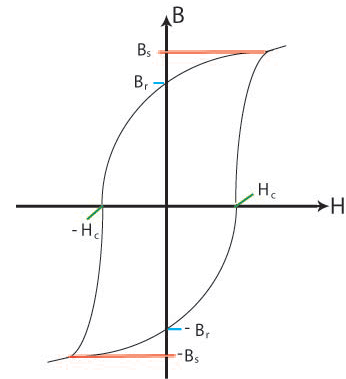
If the external applied field is removed the single domain will rotate back to the easy direction in the crystal. A demagnetising field will be set up due to the single domain, and this field initiates the formation of reverse magnetic domains as these will lower the magnetostatic energy of the sample by reducing the demagnetising field. However the demagnetising field is not strong enough for the domain walls to be able to grow past crystal defects so they can never fully reverse back to their original positions when there is no external applied field. This results in the hysteresis curve as some magnetisation will remain when there is no external applied field. This magnetisation is called the remanent magnetisation, Br. The field required to reduce the magnetisation of the sample to zero is called the coercive field Hc. And the saturation magnetisation Bs is the magnetisation when all the domains are aligned parallel to the external field. These are shown on the schematic below:

Figure S. Schematic showing the general shape of the hysteresis curve with some relevant points marked;
Bs, the saturation magnetisation; Br, the remanent magnetisation; Hc, the coercive field.
The movie clip below shows the domain structure as the material is subjected to a hysteresis cycle.
Hard and soft magnets
Ferromagnetic materials are further classified as soft or hard. Hard magnets are also called permanent magnets. These require a large field to demagnetise (and magnetise). Generally hard magnets have a large remenant magnetisation. Soft magnets, however, are easily magnetised and demagnetised, they have a small coercive field, and generally a small remanent magnetisation. Soft and hard magnets have different applications depending on the ease of magnetisation and demagnetisation required. See the animation below for examples of hard and soft magnets, their hysteresis curves and applications.


