
6.2: Stiffness of Long Fiber Composites
- Page ID
- 8200
")
\( \newcommand{\vecs}[1]{\overset { \scriptstyle \rightharpoonup} {\mathbf{#1}} } \)
\( \newcommand{\vecd}[1]{\overset{-\!-\!\rightharpoonup}{\vphantom{a}\smash {#1}}} \)
\( \newcommand{\dsum}{\displaystyle\sum\limits} \)
\( \newcommand{\dint}{\displaystyle\int\limits} \)
\( \newcommand{\dlim}{\displaystyle\lim\limits} \)
\( \newcommand{\id}{\mathrm{id}}\) \( \newcommand{\Span}{\mathrm{span}}\)
( \newcommand{\kernel}{\mathrm{null}\,}\) \( \newcommand{\range}{\mathrm{range}\,}\)
\( \newcommand{\RealPart}{\mathrm{Re}}\) \( \newcommand{\ImaginaryPart}{\mathrm{Im}}\)
\( \newcommand{\Argument}{\mathrm{Arg}}\) \( \newcommand{\norm}[1]{\| #1 \|}\)
\( \newcommand{\inner}[2]{\langle #1, #2 \rangle}\)
\( \newcommand{\Span}{\mathrm{span}}\)
\( \newcommand{\id}{\mathrm{id}}\)
\( \newcommand{\Span}{\mathrm{span}}\)
\( \newcommand{\kernel}{\mathrm{null}\,}\)
\( \newcommand{\range}{\mathrm{range}\,}\)
\( \newcommand{\RealPart}{\mathrm{Re}}\)
\( \newcommand{\ImaginaryPart}{\mathrm{Im}}\)
\( \newcommand{\Argument}{\mathrm{Arg}}\)
\( \newcommand{\norm}[1]{\| #1 \|}\)
\( \newcommand{\inner}[2]{\langle #1, #2 \rangle}\)
\( \newcommand{\Span}{\mathrm{span}}\) \( \newcommand{\AA}{\unicode[.8,0]{x212B}}\)
\( \newcommand{\vectorA}[1]{\vec{#1}} % arrow\)
\( \newcommand{\vectorAt}[1]{\vec{\text{#1}}} % arrow\)
\( \newcommand{\vectorB}[1]{\overset { \scriptstyle \rightharpoonup} {\mathbf{#1}} } \)
\( \newcommand{\vectorC}[1]{\textbf{#1}} \)
\( \newcommand{\vectorD}[1]{\overrightarrow{#1}} \)
\( \newcommand{\vectorDt}[1]{\overrightarrow{\text{#1}}} \)
\( \newcommand{\vectE}[1]{\overset{-\!-\!\rightharpoonup}{\vphantom{a}\smash{\mathbf {#1}}}} \)
\( \newcommand{\vecs}[1]{\overset { \scriptstyle \rightharpoonup} {\mathbf{#1}} } \)
\(\newcommand{\longvect}{\overrightarrow}\)
\( \newcommand{\vecd}[1]{\overset{-\!-\!\rightharpoonup}{\vphantom{a}\smash {#1}}} \)
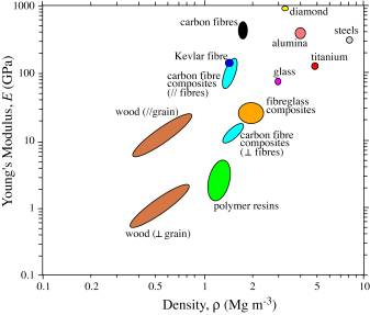
\(\newcommand{\avec}{\mathbf a}\) \(\newcommand{\bvec}{\mathbf b}\) \(\newcommand{\cvec}{\mathbf c}\) \(\newcommand{\dvec}{\mathbf d}\) \(\newcommand{\dtil}{\widetilde{\mathbf d}}\) \(\newcommand{\evec}{\mathbf e}\) \(\newcommand{\fvec}{\mathbf f}\) \(\newcommand{\nvec}{\mathbf n}\) \(\newcommand{\pvec}{\mathbf p}\) \(\newcommand{\qvec}{\mathbf q}\) \(\newcommand{\svec}{\mathbf s}\) \(\newcommand{\tvec}{\mathbf t}\) \(\newcommand{\uvec}{\mathbf u}\) \(\newcommand{\vvec}{\mathbf v}\) \(\newcommand{\wvec}{\mathbf w}\) \(\newcommand{\xvec}{\mathbf x}\) \(\newcommand{\yvec}{\mathbf y}\) \(\newcommand{\zvec}{\mathbf z}\) \(\newcommand{\rvec}{\mathbf r}\) \(\newcommand{\mvec}{\mathbf m}\) \(\newcommand{\zerovec}{\mathbf 0}\) \(\newcommand{\onevec}{\mathbf 1}\) \(\newcommand{\real}{\mathbb R}\) \(\newcommand{\twovec}[2]{\left[\begin{array}{r}#1 \\ #2 \end{array}\right]}\) \(\newcommand{\ctwovec}[2]{\left[\begin{array}{c}#1 \\ #2 \end{array}\right]}\) \(\newcommand{\threevec}[3]{\left[\begin{array}{r}#1 \\ #2 \\ #3 \end{array}\right]}\) \(\newcommand{\cthreevec}[3]{\left[\begin{array}{c}#1 \\ #2 \\ #3 \end{array}\right]}\) \(\newcommand{\fourvec}[4]{\left[\begin{array}{r}#1 \\ #2 \\ #3 \\ #4 \end{array}\right]}\) \(\newcommand{\cfourvec}[4]{\left[\begin{array}{c}#1 \\ #2 \\ #3 \\ #4 \end{array}\right]}\) \(\newcommand{\fivevec}[5]{\left[\begin{array}{r}#1 \\ #2 \\ #3 \\ #4 \\ #5 \\ \end{array}\right]}\) \(\newcommand{\cfivevec}[5]{\left[\begin{array}{c}#1 \\ #2 \\ #3 \\ #4 \\ #5 \\ \end{array}\right]}\) \(\newcommand{\mattwo}[4]{\left[\begin{array}{rr}#1 \amp #2 \\ #3 \amp #4 \\ \end{array}\right]}\) \(\newcommand{\laspan}[1]{\text{Span}\{#1\}}\) \(\newcommand{\bcal}{\cal B}\) \(\newcommand{\ccal}{\cal C}\) \(\newcommand{\scal}{\cal S}\) \(\newcommand{\wcal}{\cal W}\) \(\newcommand{\ecal}{\cal E}\) \(\newcommand{\coords}[2]{\left\{#1\right\}_{#2}}\) \(\newcommand{\gray}[1]{\color{gray}{#1}}\) \(\newcommand{\lgray}[1]{\color{lightgray}{#1}}\) \(\newcommand{\rank}{\operatorname{rank}}\) \(\newcommand{\row}{\text{Row}}\) \(\newcommand{\col}{\text{Col}}\) \(\renewcommand{\row}{\text{Row}}\) \(\newcommand{\nul}{\text{Nul}}\) \(\newcommand{\var}{\text{Var}}\) \(\newcommand{\corr}{\text{corr}}\) \(\newcommand{\len}[1]{\left|#1\right|}\) \(\newcommand{\bbar}{\overline{\bvec}}\) \(\newcommand{\bhat}{\widehat{\bvec}}\) \(\newcommand{\bperp}{\bvec^\perp}\) \(\newcommand{\xhat}{\widehat{\xvec}}\) \(\newcommand{\vhat}{\widehat{\vvec}}\) \(\newcommand{\uhat}{\widehat{\uvec}}\) \(\newcommand{\what}{\widehat{\wvec}}\) \(\newcommand{\Sighat}{\widehat{\Sigma}}\) \(\newcommand{\lt}{<}\) \(\newcommand{\gt}{>}\) \(\newcommand{\amp}{&}\) \(\definecolor{fillinmathshade}{gray}{0.9}\)Before we go into the details it is worth noting that the most suitable material for a given application may well not be the stiffest material. For example, for a given force applied to the free end of a cantilevered composite beam, the minimum deflection per unit mass is achieved by maximizing the merit index E / ρ2.
Click here for Merit index derivation. (See Optimisation of Materials Properties in Living Systems for more on merit indices)
An Ashby property map (Young's Modulus against Density) for composites:
The axial and transverse Young's Moduli can be predicted using a simple slab model, in which the fibre and matrix are represented by parallel slabs of material, with thicknesses in proportion to their volume fractions, E and (1- E).
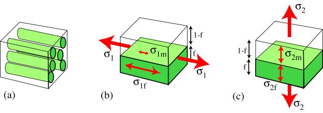
Axial Loading: Voigt model
The fibre strain is equal to the matrix strain: EQUAL STRAIN.
\[\varepsilon_{1}=\varepsilon_{1 f}=\frac{\sigma_{1 f}}{E_{f}}=\varepsilon_{1 m}=\frac{\sigma_{1 m}}{E_{m}}=\frac{\sigma_{1}}{E_{1}}\]
See definitions of terms
For a composite in which the fibres are much stiffer than the matrix ( Ef >> Em ), the reinforcement fibre is subject to much higher stresses ( σ1f >> σ1m ) than the matrix and there is a redistribution of the load. The overall stress σ1 can be expressed in terms of the two contributions:
\[\sigma_{1}=(1-f) \sigma_{1 \mathrm{m}}+f \sigma_{1 f}\]
The Young's modulus of the composite can now be written as
\[E_{1}=\frac{\sigma_{1}}{\varepsilon_{1}}=\frac{(1-f) \sigma_{1 \mathrm{m}}+f \sigma_{1 \mathrm{f}}}{\left(\frac{\sigma_{1 \mathrm{f}}}{E_{\mathrm{f}}}\right)}=(1-f) E_{\mathrm{m}}+f E_{\mathrm{f}}\]
This is known as the "Rule of Mixtures" and it shows that the axial stiffness is given by a weighted mean of the stiffnesses of the two components, depending only on the volume fraction of fibres.
Transverse Loading: Reuss Model
The stress acting on the reinforcement is equal to the stress acting on the matrix: EQUAL STRESS.
\[\sigma_{2}=\sigma_{2 f}=\varepsilon_{2 f} E_{f}=\sigma_{2 m}=\varepsilon_{2 m} E_{m}\]
The net strain is the sum of the contributions from the matrix and the fibre:
\[\varepsilon_{2}=f \varepsilon_{2 \mathrm{f}}+(1-f) \varepsilon_{2 \mathrm{m}}\]
from which the composite modulus is given by:
\[E_{2}=\frac{\sigma_{2}}{\varepsilon_{2}}=\frac{\sigma_{2 \mathrm{f}}}{f \varepsilon_{2 \mathrm{f}}+(1-f) \varepsilon_{2 \mathrm{m}}}=\left[\frac{f}{E_{\mathrm{f}}}+\frac{(1-f)}{E_{\mathrm{m}}}\right]^{-1}\]
This "Inverse Rule of Mixtures" is actually a poor approximate for E2 since in reality regions of the matrix 'in series' with the fibres, close to them and in line along the loading direction, are subjected to a high stress similar to that carried by the reinforcement fibres; whereas the regions of the matrix 'in parallel' with the fibres (adjacent laterally) are constrained to have the same strain as the fibres and carry a low stress. This leads to non-uniform distributions of stress and strain during transverse loading, which means that the model is inappropriate. The slab model provides the lower bound for the transverse stiffness.
A more successful estimate is the semi-empirical Halpin-Tsai expression:
\[E_{2}=\frac{E_{m}(1+\xi \eta f)}{(1-\eta f)}\]
where
\[\eta=\frac{\left(\frac{E_{f}}{E_{m}}-1\right)}{\left(\frac{E_{f}}{E_{m}}+\xi\right)} \text { and } \xi \approx 1\]
An even more powerful, but complex, analytical tool is the Eshelby method (see Hull and Clyne, 1996).