
4.2: General Properties of the Beam Governing Equation- General and Particular Solutions
- Page ID
- 21491
\( \newcommand{\vecs}[1]{\overset { \scriptstyle \rightharpoonup} {\mathbf{#1}} } \)
\( \newcommand{\vecd}[1]{\overset{-\!-\!\rightharpoonup}{\vphantom{a}\smash {#1}}} \)
\( \newcommand{\dsum}{\displaystyle\sum\limits} \)
\( \newcommand{\dint}{\displaystyle\int\limits} \)
\( \newcommand{\dlim}{\displaystyle\lim\limits} \)
\( \newcommand{\id}{\mathrm{id}}\) \( \newcommand{\Span}{\mathrm{span}}\)
( \newcommand{\kernel}{\mathrm{null}\,}\) \( \newcommand{\range}{\mathrm{range}\,}\)
\( \newcommand{\RealPart}{\mathrm{Re}}\) \( \newcommand{\ImaginaryPart}{\mathrm{Im}}\)
\( \newcommand{\Argument}{\mathrm{Arg}}\) \( \newcommand{\norm}[1]{\| #1 \|}\)
\( \newcommand{\inner}[2]{\langle #1, #2 \rangle}\)
\( \newcommand{\Span}{\mathrm{span}}\)
\( \newcommand{\id}{\mathrm{id}}\)
\( \newcommand{\Span}{\mathrm{span}}\)
\( \newcommand{\kernel}{\mathrm{null}\,}\)
\( \newcommand{\range}{\mathrm{range}\,}\)
\( \newcommand{\RealPart}{\mathrm{Re}}\)
\( \newcommand{\ImaginaryPart}{\mathrm{Im}}\)
\( \newcommand{\Argument}{\mathrm{Arg}}\)
\( \newcommand{\norm}[1]{\| #1 \|}\)
\( \newcommand{\inner}[2]{\langle #1, #2 \rangle}\)
\( \newcommand{\Span}{\mathrm{span}}\) \( \newcommand{\AA}{\unicode[.8,0]{x212B}}\)
\( \newcommand{\vectorA}[1]{\vec{#1}} % arrow\)
\( \newcommand{\vectorAt}[1]{\vec{\text{#1}}} % arrow\)
\( \newcommand{\vectorB}[1]{\overset { \scriptstyle \rightharpoonup} {\mathbf{#1}} } \)
\( \newcommand{\vectorC}[1]{\textbf{#1}} \)
\( \newcommand{\vectorD}[1]{\overrightarrow{#1}} \)
\( \newcommand{\vectorDt}[1]{\overrightarrow{\text{#1}}} \)
\( \newcommand{\vectE}[1]{\overset{-\!-\!\rightharpoonup}{\vphantom{a}\smash{\mathbf {#1}}}} \)
\( \newcommand{\vecs}[1]{\overset { \scriptstyle \rightharpoonup} {\mathbf{#1}} } \)
\(\newcommand{\longvect}{\overrightarrow}\)
\( \newcommand{\vecd}[1]{\overset{-\!-\!\rightharpoonup}{\vphantom{a}\smash {#1}}} \)
\(\newcommand{\avec}{\mathbf a}\) \(\newcommand{\bvec}{\mathbf b}\) \(\newcommand{\cvec}{\mathbf c}\) \(\newcommand{\dvec}{\mathbf d}\) \(\newcommand{\dtil}{\widetilde{\mathbf d}}\) \(\newcommand{\evec}{\mathbf e}\) \(\newcommand{\fvec}{\mathbf f}\) \(\newcommand{\nvec}{\mathbf n}\) \(\newcommand{\pvec}{\mathbf p}\) \(\newcommand{\qvec}{\mathbf q}\) \(\newcommand{\svec}{\mathbf s}\) \(\newcommand{\tvec}{\mathbf t}\) \(\newcommand{\uvec}{\mathbf u}\) \(\newcommand{\vvec}{\mathbf v}\) \(\newcommand{\wvec}{\mathbf w}\) \(\newcommand{\xvec}{\mathbf x}\) \(\newcommand{\yvec}{\mathbf y}\) \(\newcommand{\zvec}{\mathbf z}\) \(\newcommand{\rvec}{\mathbf r}\) \(\newcommand{\mvec}{\mathbf m}\) \(\newcommand{\zerovec}{\mathbf 0}\) \(\newcommand{\onevec}{\mathbf 1}\) \(\newcommand{\real}{\mathbb R}\) \(\newcommand{\twovec}[2]{\left[\begin{array}{r}#1 \\ #2 \end{array}\right]}\) \(\newcommand{\ctwovec}[2]{\left[\begin{array}{c}#1 \\ #2 \end{array}\right]}\) \(\newcommand{\threevec}[3]{\left[\begin{array}{r}#1 \\ #2 \\ #3 \end{array}\right]}\) \(\newcommand{\cthreevec}[3]{\left[\begin{array}{c}#1 \\ #2 \\ #3 \end{array}\right]}\) \(\newcommand{\fourvec}[4]{\left[\begin{array}{r}#1 \\ #2 \\ #3 \\ #4 \end{array}\right]}\) \(\newcommand{\cfourvec}[4]{\left[\begin{array}{c}#1 \\ #2 \\ #3 \\ #4 \end{array}\right]}\) \(\newcommand{\fivevec}[5]{\left[\begin{array}{r}#1 \\ #2 \\ #3 \\ #4 \\ #5 \\ \end{array}\right]}\) \(\newcommand{\cfivevec}[5]{\left[\begin{array}{c}#1 \\ #2 \\ #3 \\ #4 \\ #5 \\ \end{array}\right]}\) \(\newcommand{\mattwo}[4]{\left[\begin{array}{rr}#1 \amp #2 \\ #3 \amp #4 \\ \end{array}\right]}\) \(\newcommand{\laspan}[1]{\text{Span}\{#1\}}\) \(\newcommand{\bcal}{\cal B}\) \(\newcommand{\ccal}{\cal C}\) \(\newcommand{\scal}{\cal S}\) \(\newcommand{\wcal}{\cal W}\) \(\newcommand{\ecal}{\cal E}\) \(\newcommand{\coords}[2]{\left\{#1\right\}_{#2}}\) \(\newcommand{\gray}[1]{\color{gray}{#1}}\) \(\newcommand{\lgray}[1]{\color{lightgray}{#1}}\) \(\newcommand{\rank}{\operatorname{rank}}\) \(\newcommand{\row}{\text{Row}}\) \(\newcommand{\col}{\text{Col}}\) \(\renewcommand{\row}{\text{Row}}\) \(\newcommand{\nul}{\text{Nul}}\) \(\newcommand{\var}{\text{Var}}\) \(\newcommand{\corr}{\text{corr}}\) \(\newcommand{\len}[1]{\left|#1\right|}\) \(\newcommand{\bbar}{\overline{\bvec}}\) \(\newcommand{\bhat}{\widehat{\bvec}}\) \(\newcommand{\bperp}{\bvec^\perp}\) \(\newcommand{\xhat}{\widehat{\xvec}}\) \(\newcommand{\vhat}{\widehat{\vvec}}\) \(\newcommand{\uhat}{\widehat{\uvec}}\) \(\newcommand{\what}{\widehat{\wvec}}\) \(\newcommand{\Sighat}{\widehat{\Sigma}}\) \(\newcommand{\lt}{<}\) \(\newcommand{\gt}{>}\) \(\newcommand{\amp}{&}\) \(\definecolor{fillinmathshade}{gray}{0.9}\)Recall from the Calculus that solution of the inhomogeneous, linear ordinary differential equation is a sum of the general solution of the homogeneous equation \(w_g\) and the particular solution of the inhomogeneous equation \(w_p\). The property of homogeneity means that \(f(Ax) = Af(x)\). The homogeneous counterpart of Equation (4.1.11) is
\[EI \frac{d^4w}{dx^4} = 0 \quad \text{ or } \quad \frac{d^4w}{dx^4} = 0 \label{4.2.1}\]
and its solution, obtained by four integrations is the third order polynomial
\[w_g(x) = \frac{C_1x^3}{6} + \frac{C_2x^2}{2} + C_3x + C_4 \label{4.2.2}\]
The particular solution \(w_p\) of the beam deflection equation, Equation (4.1.11) depends on the loading, but not the boundary conditions. For the uniformly loaded beam the particular solution is the first term in Equation (4.1.27-4.1.28). As an illustration, consider the same pin-pin supported beam loaded by the triangular line load
\[q(x) = q_0 \frac{2x}{l} \; , \; 0 < x < \frac{l}{2}\]
where \(q_0\) is the load intensity at mid-span \(x = l/2\). The particular solution of this problem, satisfying the governing equation is
\[w_p = \frac{q_0x^5}{60EIl}\]
Then, the full solution is \(w(x) = w_g + w_p\).
Beam loaded by concentrated forces (or moments) requires special consideration.
Continuity requirements
A sudden change in the beam cross-section or loading may produce a discontinuous solution. What quantities may suffer a jump and what must be continuous?
In mechanics the discontinuity of a given function is denoted by a square bracket
\[[f(\xi)] = f(\xi^+) − f(\xi^-)\]
where \(\xi^+\) and \(\xi^-\) denote the values of the argument on the right and left hand of a discontinuity. In the quasi-static theory of beam
\[[w] = 0 \label{4.2.6}\]
\[\left[\frac{dw}{dx}\right] = 0\]
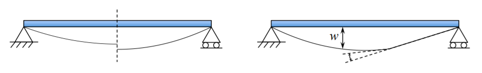
The discontinuity in the vertical displacement means separation so of course it may not occur. Why then slopes must be continuous for elastic beams? This is simple. A change of slope is called a curvature. A jump in the slope gives an infinite curvature, and thus an infinite bending moments. Such a situation is impossible, because the beam cross-section will go into plastic range, and the beam will no longer stay elastic. Quantities that can be discontinuous are
\[\text{Bending monents } \quad [M] = \bar{M} \]
\[\text{Shear force } \quad [V] = \bar{V} \label{4.2.9}\]
As an illustration, consider a pin-pin supported beam loaded at mid-span by a point force \(P\).
As mentioned earlier, the point load can be considered as a limiting case of a continuous line load with the help of the Dirac delta function
\[q(x) = P \delta(x − \frac{l}{2}), \quad \text{ where } \int \delta(x − \frac{l}{2})dx = 1 \]
Even though techniques have been developed to deal with singularity functions for beams, they require to use the apparatus of the mathematical theory of distribution. This
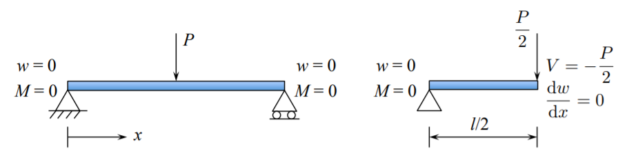
is not the avenue that we will take. instead, a symmetry boundary condition will be imposed. Now, the concentrated load is not applied inside the beam \(0 < x < l\), governed by the inhomogeneous differential equation, but at the boundary. Each half of the beam is carrying half of the load. Therefore, the boundary conditions are
\[\text { at } x = 0 \; w = 0 \]
\[ \frac{d^{2} w}{d x^{2}} = 0\]
\[\text { at } x = \frac{l}{2} \; V= -\frac{P}{2} \]
\[ \frac{d w}{d x} = 0\]
Because the loading is applied on the boundary, the differential equation becomes homogeneous. The solution of Equation \ref{4.2.1} is given by the third order polynomial, substituting the above BC into the solution given by Equation \ref{4.2.2}, a system of four linear algebraic equations is obtained, where the solution is
\[C_1 = − \frac{D}{2EI} , \; C_2 = 0, \; C_3 = \frac{Pl^2}{16EI}, \; C_4 = 0 \]
The deflection line is given by
\[w(x) = \frac{P x}{48EI} (3l^2 − 4x^2 )\]
and the central deflection (something to remember) is
\[w_0 = w(x = \frac{l}{2} ) = \frac{pl^3}{48EI}\]
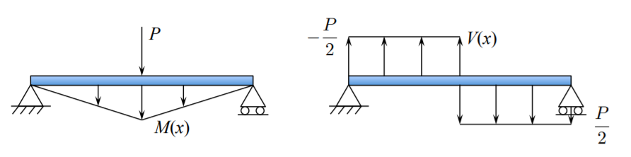
The plot of the distribution of bending moment and shear forces along the length of the beam determined from the calculated deflection line is shown in Figure (\(\PageIndex{3}\)).
Note that the jump in the internal shear force is equal to the applied force
\[[V ] = V_{\text{right}}(x = \frac{l}{2}) − V_{\text{left}}(x = \frac{l}{2}) = P\]
If the point load is not applied at the mid-span but at an arbitrary distance \(x = a\), the beam must be divided into two parts \(0 < x < a\), \(a < x < l\), and each part must be solved independently.
\[\text{First segment } 0 < x < a \; w^{\mathrm{I}}(x) = \frac{C_1x^3}{6} + \frac{C_2x^2}{2} + C_3x + C_4\]
\[\text{Second segment } a < x < l \; w^{\mathrm{II}}(x) = \frac{C_5x^3}{6} + \frac{C_6x^2}{2} + C_7x + C_8\]
This gives rise to eight integration constants, four for each side. Would there be enough conditions to determine these constants? The answer is YES. There are two boundary conditions at \(x = 0\), four continuity conditions at \(x = a\), given by Equations \ref{4.2.6}-\ref{4.2.9} and, again, two boundary conditions at \(x = l\). In summary
\[\begin{array}{l|l|l}
\mathrm{BC}, x = 0 & \text { Continuity, } x = a & \mathrm{BC}, x = l \\
\hline w = 0 & {[w] = 0} & w = 0 \\
M = 0 & {\left[ \frac{d w}{d x} \right] = 0} & M=0 \\
& {[M] = 0} \\
& {[V] = P}
\end{array}\]
Note that there is no concentrated bending moment applied \(\bar{M} = 0\) so that the bending moment field is continueous across \(x = a\). The concentrated force produces a jump in the distribution of the shear forces, so \(\bar{V} = P\).
We leave it to the reader to apply the above condition and solve the problem. More on this problem can be found in two sections of this notes: Problem Sets and Recitations.
The method of superposition says that the deflections and slopes of the beam subjected to a system of loads are equal to the sum of those quantities due to individual loads. In other words the individual results may be superimposed to determine a combined response, hence the term method of superposition.
This is a very powerful and convenient method since solutions for many support and loading conditions are readily available in various engineering handbooks. Using the principle of superposition, we may combine these solutions to obtain a solution for more complicated loading conditions.
As an example, consider a clamped-clamped beam loaded by a uniform line load \(q\) and concentrated force at the center \(P\). The deflection formulas for the two individual loading are
\[w|_{\text{uniform}} = \frac{qx^2}{24EI} (l − x)^2\]
\[w|_{\text{point}} = \frac{Px^2}{48EI} (3l − 4x)\]
The solution for both loads acting together is
\[w_{\text{total}} = w|_{\text{uniform}} + w|_{\text{point}}\]