7.3: Deflection by Method of Double Integration

Deflection by double integration is also referred to as deflection by the method of direct or constant integration. This method entails obtaining the deflection of a beam by integrating the differential equation of the elastic curve of a beam twice and using boundary conditions to determine the constants of integration. The first integration yields the slope, and the second integration gives the deflection. This method is best when there is a continuity in the applied loading.

Example 7.1

A cantilever beam is subjected to a combination of loading, as shown in Figure 7.2a. Using the method of double integration, determine the slope and the deflection at the free end.

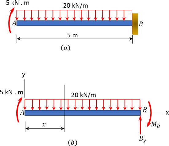
\(Fig. 7.2\). Cantilever beam.

Solution

Equation for bending moment. Passing a section at a distance \(x\) from the free-end of the beam, as shown in the free-body diagram in Figure 7.2b, and considering the moment to the right of the section suggests the following:

\(M=5-\frac{20 x^{2}}{2}\)

Substituting \(M\) into equation 7.12 suggests the following:

\(E I \frac{d^{2} y}{d x^{2}}=5-\frac{20 x^{2}}{2}\)

Equation for slope. Integrating with respect to \(x\) suggests the following:

\(E I \frac{d y}{d x}=5 x-\frac{20 x^{3}}{6}+C_{1}\)

Observe that at the fixed end where \(x=L\), \(\frac{d y}{d x}=0\); this is referred to as the boundary condition. Applying these boundary conditions to equation 3 suggests the following:

\(\begin{array}{l}
0=5 L-\frac{20 \mathrm{~L}^{3}}{6}+C_{1} \\
C_{1}=-5 \times 5+\frac{20(5)^{3}}{6}=391.67
\end{array}\)

To obtain the following equation of slope, substitute the computed value of \(C_{1}\) into equation 3 follows:

\(E I \frac{d y}{d x}=5 x-\frac{20 x^{3}}{6}+391.67\)

Equation for deflection. Integrating equation 4 suggests the following:

\(\text { EIy }=\frac{5 x^{2}}{2}-\frac{20 x^{4}}{24}+391.67 x+C_{2}\)

At the fixed end \(x=L\), \(y = 0\). Applying these boundary conditions to equation 5 suggests the following:

\(0=\frac{5(L)^{2}}{2}-\frac{20(L)^{4}}{24}+391.67 L=\frac{5(5)^{2}}{2}-\frac{20(5)^{4}}{24}+391.67(5)+C_{2}=-1500\)

To obtain the following equation of elastic curve, substitute the computed value of \(C_{2}\) into equation 5, as follows:

\(y=\frac{1}{E I}\left(\frac{5 x^{2}}{2}-\frac{20 x^{4}}{24}+391.67 x-1500\right)\)

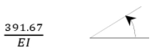
The slope at the free end, i.e., \(\frac{d y}{d x}\) at \(x = 0\)

\(\left(\frac{d y}{d x}\right)_{\mathrm{A}}=\theta_{\mathrm{A}}=\frac{1}{E I}\left[5(0)-\frac{20(0)^{3}}{6}+391.6\right]=\frac{391.67}{E I}\)

The deflection at the free end, i.e., \(y\) at \(x = 0\)

\(y_{\mathrm{A}}=\frac{1}{E I}\left(\frac{5(0)^{2}}{2}-\frac{20(0)^{4}}{24}+391.67(0)-1500\right)=-\frac{1500}{E I} \quad \frac{1500}{E I} \downarrow\)

Example 7.2

A simply supported beam \(AB\) carries a uniformly distributed load of 2 kips/ft over its length and a concentrated load of 10 kips in the middle of its span, as shown in Figure 7.3a. Using the method of double integration, determine the slope at support \(A\) and the deflection at a midpoint \(C\) of the beam.

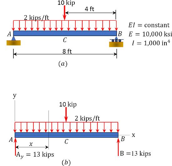
\(Fig. 7.3\). Simply supported beam.

Solution

Support reactions.

\(A_{y}=B_{y}=\frac{2 \times 8}{2}+\frac{10}{2}=13\) kips by symmetry

Equation for bending moment. The moment at a section of a distance \(x\) from support \(A\), as shown in the free-body diagram in Figure 7.3b, is written as follows:

\(0<x<4\)

\(M=13 x-\frac{2 x^{2}}{2}\)

Substituting for \(M\) into equation 7.12 suggests the following:

\(E I \frac{d^{2} y}{d x^{2}}=M=13 x-\frac{2 x^{2}}{2}\)

Equation for slope. Integrating equation 2 with respect to \(x\) suggests the following:

\(E I \frac{d y}{d x}=\frac{13 x^{2}}{2}-\frac{2 x^{3}}{6}+C_{1}\)

The constant of integration \(C_{1}\) is evaluated by considering the boundary condition.

\(\text { At } x=\frac{L}{2}, \frac{d y}{d x}=0\)

Applying the afore-stated boundary conditions to equation 3 suggests the following:

\(\begin{array}{l}
0=\frac{13(4)^{2}}{2}-\frac{2(4)^{3}}{6}+C_{1} \\
C_{1}=-82.67
\end{array}\)

Bringing the computed value of \(C_{1}\) back into equation 3 suggests the following:

\(\frac{d y}{d x}=\frac{1}{E I}\left(\frac{13 x^{2}}{2}-\frac{2 x^{3}}{6}-82.67\right)\)

Equation for deflection. Integrating equation 4 suggests the following:

\(\text { EIy }=\frac{13 x^{3}}{6}-\frac{2 x^{4}}{24}-82.67 x+C_{2}\)

The constant of integration \(C_{2}\) is evaluated by considering the boundary condition.

At \(x =0\), \(y = 0\)

\(0=0-0-0+C_{2}\)

\(C_{2}=0\)

Carrying the computed value of \(C_{2}\) back into equation 5 suggests the following equation of elastic curve:

\(\text { EIy }=\frac{13 x^{3}}{6}-\frac{2 x^{4}}{24}-82.67 x\)

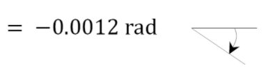
The slope at \(A\), i.e., \(\frac{d y}{d x}\) at \(x = 0\)

\(\left(\frac{d y}{d x}\right)_{\mathrm{A}}=\theta_{\mathrm{A}}=\frac{1}{E I}\left(\frac{13(0)^{2}}{2}-\frac{2(0)^{3}}{6}-82.67\right)=-\frac{82.67}{E I}=-\frac{82.67}{(10,000)(12)^{2}\left(\frac{1000}{(12)^{4}}\right)}\)

Deflection at midpoint \(C\), i.e., at \(x=\frac{L}{2}\)

\(\begin{aligned}
y_{c} &=\frac{1}{E I}\left[\frac{13(4)^{3}}{6}-\frac{2(4)^{4}}{24}-82.67(4)\right]=-\frac{213.35}{E I}=-\frac{213.35}{(10,000)(144)(1000)\left(12^{-4}\right)} \\
&=-0.0031 \mathrm{ft}=-0.04 \mathrm{in} \downarrow
\end{aligned}\)

Example 7.3

A beam carries a distributed load that varies from zero at support \(A\) to 50 kN/m at its overhanging end, as shown in Figure 7.4a. Write the equation of the elastic curve for segment \(AB\) of the beam, determine the slope at support \(A\), and determine the deflection at a point of the beam located 3 m from support \(A\).

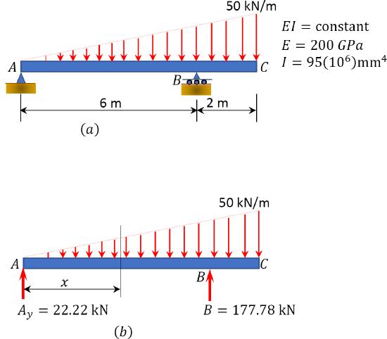
\(Fig. 7.4\). Beam.

Solution

Support reactions. To determine the reactions of the beam, apply the equations of equilibrium, as follows:

\(\begin{array}{l}
+n \sum M_{A}=0 \\
-\left(\frac{1}{2}\right)(8)(50)\left(\frac{2}{3}\right)(8)+B_{y}(6)=0 \\
B_{y}=177.78 \mathrm{kN} \quad \quad B_{y}=177.78 \uparrow \\
+\rightarrow \sum F_{x}=0 \quad A_{x}=0 \quad \quad A_{x} = 0 \\
+\uparrow \sum F_{\mathrm{y}}=0 \\
177.78+A_{y}-\left(\frac{1}{2}\right)(8)(50)=0 \\
A_{y}=22.22 \mathrm{kN} \quad \quad A_{y}=22.22 \mathrm{kN} \uparrow
\end{array}\)

Equation for bending moment. The moment at a section of a distance \(x\) from support \(A\), as shown in the free-body diagram in Figure 7.4b, is as follows:

\(0 < x < 6\)

\(M=22.22 x-\left(\frac{1}{2}\right)(x)\left(\frac{50 x}{8}\right)\left(\frac{x}{3}\right)=22.22 x-\frac{25 x^{3}}{24}\)

Substituting for \(M\) into equation 7.12 suggests the following:

\(E I \frac{d^{2} y}{d x^{2}}=M=2.22 x-\frac{25 x^{3}}{24}\)

Equation for slope. Integrating equation 2 with respect to \(x\) suggests the following:

\(E I \frac{d y}{d x}=\frac{22.22 x^{2}}{2}-\frac{25 x^{4}}{4 \times 24}+C_{1}\)

Equation for deflection. Integrating equation 3 suggests the equation of deflection, as follows:

\(\text { EIy }=\frac{22.22 x^{3}}{6}-\frac{25 x^{5}}{5 \times 4 \times 24}+C_{1} x+C_{2}\)

To evaluate the constants of integrations, apply the following boundary conditions to equation 4:

At \(x = 0\), \(y = 0\)

\(0=0-0+0+C_{2}\)

\(C_{2}=0\)

At \(x = 6\) m, \(y = 0\)

\(0=\frac{22.22(6)^{3}}{6}-\frac{25(6)^{5}}{5 \times 4 \times 24}+6 C_{1}\)

\(C_{1}=-65.82\)

Equation of elastic curve.

The equation of elastic curve can now be determined by substituting \(C_{1}\) and \(C_{2}\) into equation 4.

\(\text { EIy }=\frac{22.22 x^{3}}{6}-\frac{25 x^{5}}{5 \times 4 \times 24}-65.82 x\)

To obtain the equations of slope and deflection, substitute the computed value of \(C_{1}\) and \(C_{2}\) back into equations 3 and 4:

Equation of slope.

\(\frac{d y}{d x}=\frac{1}{E I}\left(\frac{22.22 x^{2}}{2}-\frac{25 x^{4}}{96}-65.82\right)\)

Equation of deflection.

\(y=\frac{1}{E I}\left(\frac{22.22 x^{3}}{6}-\frac{25 x^{5}}{480}-65.82 x\right)\)

Deflection at \(x = 3\) m from support \(A\).

\(\mathrm{y}_{x}=3 \mathrm{~m}=-\frac{110.13}{E I}=-0.0058 \mathrm{~m}=-5.80 \mathrm{~mm} \quad 5.80 \mathrm{~mm} \downarrow\)