7.4: Deflection by Method of Singularity Function

In cases where a beam is subjected to a combination of distributed loads, concentrated loads, and moments, using the method of double integration to determine the deflections of such beams is really involving, since various segments of the beam are represented by several moment functions, and much computational efforts are required to find the constants of integration. Using the method of singularity function in such cases to determine deflections is comparatively easier and relatively quick. This method of analysis was first introduced by Macaulay in 1919, and it entails the use of one equation that contains a singularity or half-range function to describe the entire beam deflection curve. A singularity or half-range function is defined as follows:

\(\langle x-a\rangle^{n}=\left\{\begin{aligned}
0 \text { for }(x-a)<0 \text { or } x<a \\
(x-a)^{n} \text { for } x-a \geq 0 & \text { or } x \geq a
\end{aligned}\right.\)

where

\(x =\) coordinate position of a point along the beam.

\(a =\) any location along the beam where discontinuity due to bending occurs.

\(n =\) the exponential values of the functions; this must always be greater than or equal to zero for the functions to be valid.

The above outlined definition implies that the quantity (\(x-a\)) equals zero or vanishes if it is negative, but it is equal to (\(x-a\)) if it is positive.

Procedure for Analysis by Singularity Function Method

•Sketch the free-body diagram of the beam and establish the \(x\) and \(y\) coordinates.

•Calculate the support reactions and write the moment equation as a function of the \(x\) coordinate. The sign convention for the moment is the same as in section 4.3.

•Substitute the moment expression into the equation of the elastic curve and integrate once to obtain the slope. Integrate again to obtain the deflection in the beam.

•Using the boundary conditions, determine the integration constants and substitute them into the equations obtained in step 3 to obtain the slope and the deflection of the beam. A positive slope is counterclockwise and a negative slope is clockwise, while a positive deflection is upward and a negative deflection is downward.

•When computing the slope or deflection at any point on the beam, discard the quantity (\(x-a\)) from the equation for slope or deflection if it is negative. If (\(x-a\)) is positive, it remains in the equation.

Example 7.4

A simply supported beam is subjected to the combined loading shown in Figure 7.5a. Using the method of singularity function, determine the slope at support \(A\) and the deflection at \(B\).

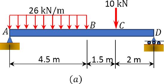
\(Fig. 7.5\). Simply supported beam.

Solution

Support reactions. To determine the reaction at support \(A\) of the beam, apply the equations of equilibrium, as follows:

\(\begin{array}{l}
+\curvearrowleft \sum M_{D}=0 \\
26(4.5)\left(8-\frac{4.5}{2}\right)+10(2)-8 A_{y}=0 \\
A_{y}=86.6 \mathrm{kN}
\end{array}\)

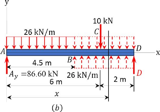
Bending moment. Replacing the given distributed load by two equivalent open-ended loadings, as shown in Figure 7.5b, the bending moment at a section located at a distance \(x\) from the left support \(A\) can be expressed as follows:

\(M=86.6 x-\frac{26 x^{2}}{2}+\frac{26(x-4.5)^{2}}{2}-10\langle x-6\rangle\)

Equation of the elastic curve. Substituting for \(M(x)\) from equation 1 into equation 7.12 suggests the following:

\(E I \frac{d^{2} y}{d x^{2}}=M=86.6 x-\frac{26 x^{2}}{2}+\frac{26(x-4.5)^{2}}{2}-10\langle x-6\rangle^{1}\)

Integrating equation 2 twice suggests the following:

\(E I \frac{d y}{d x}=\frac{86.6 x^{2}}{2}-\frac{26 x^{3}}{3 \times 2}+\frac{26(x-4.5)^{3}}{3 \times 2}-\frac{10(x-6)^{2}}{2}+C_{1}\)

\(EIy=\frac{86.6 x^{3}}{3 \times 2}-\frac{26 x^{4}}{4 \times 3 \times 2}+\frac{26(x-4.5)^{4}}{4 \times 3 \times 2}-\frac{10\langle x-6\rangle^{3}}{3 \times 2}+C_{1} x+C_{2}\)

Boundary conditions and computation of constants of integration. Applying the boundary conditions \([x=0, y=0]\) to equation 4 and noting that each bracket contains a negative quantity and, thus, is equal zero by the singularity definition suggests that \(C_{2} = 0\).

\(0=0-0+0-0+C_{2}\)

\(C_{2} = 0\)

Again, applying the boundary conditions \([x=8, y=0]\) to equation 4 and noting that each bracket contains a positive quantity suggests that the value of the constant \(C_{1}\) is as follows:

\(\begin{array}{l}
0=\frac{86.6(8)^{3}}{3 \times 2}-\frac{26(8)^{4}}{4 \times 3 \times 2}+\frac{26(8-4.5)^{4}}{4 \times 3 \times 2}-\frac{10(8-6)^{3}}{3 \times 2}+8 C_{1} \\
C_{1}=-387.72
\end{array}\)

\(\begin{array}{l}
0=\frac{86.6(8)^{3}}{3 \times 2}-\frac{26(8)^{4}}{4 \times 3 \times 2}+\frac{26(8-4.5)^{4}}{4 \times 3 \times 2}-\frac{10(8-6)^{3}}{3 \times 2}+8 C_{1} \\
C_{1}=-387.72
\end{array}\)

Substituting the values for \(C_{1}\) and \(C_{2}\) into equation 4 suggets that the expression for the elastic curve of the beam is as follows:

\[y=\frac{1}{E I}\left\{\frac{86.6 x^{3}}{6}-\frac{26 x^{4}}{24}+\frac{26(x-4.5)^{4}}{24}-\frac{10\langle x-6\rangle^{3}}{6}-387.72 x\right\}\]

Similarly, substituting the values for \(C_{1}\) into equation 3 suggests the expression for the slope is as follows:

\[\frac{d y}{d x}=\frac{1}{E I}\left\{\frac{86.6 x^{2}}{2}-\frac{26 x^{3}}{6}+\frac{26(x-4.5)^{3}}{6}-\frac{10(x-6)^{2}}{2}-387.72\right\}\]

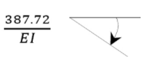
The slope at \(A\), i.e., \(\frac{d y}{d x}\) at \(x = 0\)

\(\left(\frac{d y}{d x}\right)_{\mathrm{A}}=\theta_{\mathrm{A}}=-\frac{387.72}{E I}\)

The deflection at \(x = 4.5\) m from support \(A\)

\(\begin{aligned}
&y_{x}=4.5 \mathrm{~m}=\frac{1}{E I}\left\{\frac{86.6(4.5)^{3}}{6}-\frac{26(4.5)^{4}}{24}+\frac{26\langle 4.5-4.5\rangle^{4}}{24}-\frac{10\langle 4.5-6\rangle^{3}}{6}-387.72(4.5)\right\}\\
&y_{x}=4.5 \mathrm{~m}=-\frac{873.74}{E I} \quad \quad \frac{873.74}{E I} \downarrow
\end{aligned}\)

Example 7.5

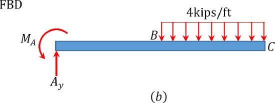
A cantilever beam is loaded with a uniformly distributed load of 4 kips/ft, as shown in Figure 7.6a. Using the method of singularity function, determine the equation of the elastic curve of the beam, the slope at the free end, and the deflection at the free end.

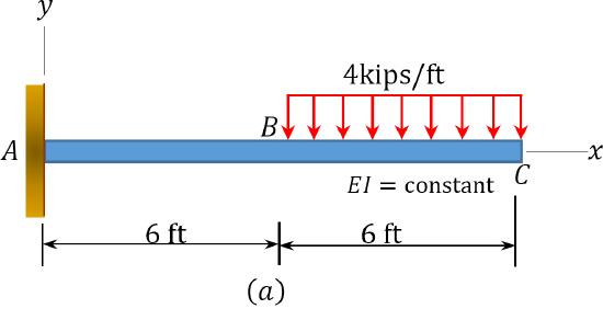
\(Fig. 7.6\). Cantilever beam.

Solution

Support reactions. To determine the reaction at support A of the beam, apply the equation of equilibrium, as follows:

\(\begin{array}{lll}
+\curvearrowleft \sum M_{A}=0 & M_{A}-4(6)(9)=0 & M_{A}=216 \mathrm{k-ft.}^{\curvearrowleft} \\
+\uparrow \sum F_{y}=0 & A_{y}-4(6)=0 & A_{y}=24 \mathrm{k} \uparrow \\
+\rightarrow \sum F_{x}=0 & A_{x}=0 & A_{x}=0
\end{array}\)

Bending moment. The bending moment at a section located at a distance \(x\) from the fixed end of the beam, shown in Figure 7.6b, can be expressed as follows:

\[M=24 x-216-\frac{4(x-6)^{2}}{2}\]

Equation of the elastic curve. Substituting for \(M(x)\) from equation 1 into equation 7.12 suggests the following:

\[E I \frac{d^{2} y}{d x^{2}}=M=24 x-216-\frac{4(x-6)^{2}}{2}\]

Integrating equation 2 twice suggests the following:

 

\[EIy=\frac{24(x)^{3}}{6}-\frac{216(x)^{2}}{2}-\frac{4(x-6)^{4}}{24}+C_{1} x+C_{2}\]

Boundary conditions and computation of constants of integration. Applying the boundary conditions \(\left[x=0, \frac{d y}{d x}=0\right]\) to equation 3 and noting that the term with a bracket contains a negative quantity and, thus, is equal to zero by the singularity function definition suggests that \(C_{1} = 0\).

\(\frac{24(0)^{2}}{2}-216(0)-\frac{4(0-6)^{3}}{6}+C_{1}=0 \quad C_{1}=0\)

Applying the boundary conditions \([x=0, y=0]\) to equation 4 and noting that the term with a bracket contains a negative quantity and, thus, is equal to zero by the singularity function definition suggests that \(C_{2} = 0\).

\(\frac{24(0)^{3}}{6}-\frac{216(0)^{2}}{2}-\frac{4(0-6)^{4}}{24}+C_{1}(0)+C_{2}=0 \quad C_{2}=0\)

To find the elastic curve of the beam, substitute the values for \(C_{1}\) and \(C_{2}\) into equation 4, as follows:

\[y=\frac{1}{E I}\left[\frac{24(x)^{3}}{6}-\frac{216(x)^{2}}{2}-\frac{4(x-6)^{4}}{24}\right]\]

Similarly, to find the expression for the slope, substitute the values for \(C_{1}\) into equation 3, as follows:

 

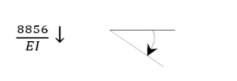
\(\left(\frac{d y}{d x}\right)_{C}=\theta_{\mathrm{C}}=\frac{1}{E I}\left[\frac{24(12)^{2}}{2}-216(12)-\frac{4(12-6)^{3}}{6}\right]=-\frac{1008}{E I} \quad \frac{1008}{E I}\)

\(y_{C}=\frac{1}{E I}\left[\frac{24(12)^{3}}{6}-\frac{216(12)^{2}}{2}-\frac{4(12-6)^{4}}{24}\right]=\frac{-8856}{E I}\)

Example 7.6

A beam with an overhang is subjected to a combined loading, as shown in Figure 7.7a. Using the method of the singularity function, determine the slope at support \(A\) and the deflection at \(B\).

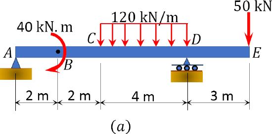
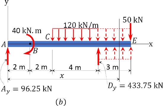
\(Fig. 7.7\). Beam with overhang.

Solution

Support reactions. To determine the reaction at support \(A\) of the beam, apply the equations of equilibrium, as follows:

\(\begin{array}{l}
+\curvearrowleft \sum M_{A}=0 \\
-40-120(4)(6)-50(11)+8 D_{y}=0 \\
D_{y}=433.75 \mathrm{kN} \quad D_{y}=433.75 \mathrm{kN} \uparrow \\
+\uparrow \sum F_{y}=0 \\
A_{y}+433.75-120(4)-50=0 \\
A_{y}=96.25 \mathrm{kN} \quad A_{y}=96.25 \mathrm{kN} \uparrow\\
+\rightarrow \sum F_{x}=0 \text { } A_{x}=0 \quad A_{x}=0
\end{array}\)

Bending moment. By replacing the given distributed load by two equivalent open-ended loadings and modifying the moment term, as shown in Figure 7.7b, the bending moment at a section located at a distance \(x\) from the left support \(A\) can be expressed as follows:

\[M=96.25 x+40\langle x-2\rangle^{0}-\frac{120(x-4)^{2}}{2}+\frac{120(x-8)^{2}}{2}+433.75\langle x-8\rangle\]

Equation of the elastic curve. Substituting for \(M(x)\) from equation 1 into equation 7.12 suggests the following:

\[E I \frac{d^{2} y}{d x^{2}}=M=96.25 x+40\langle x-2\rangle^{0}-\frac{120(x-4)^{2}}{2}+\frac{120\langle x-8\rangle^{2}}{2}+433.75\langle x-8\rangle\]

Integrating equation 2 twice suggests the following:

\[E I \frac{d y}{d x}=\frac{96.25 x^{2}}{2}+40\langle x-2\rangle^{1}-\frac{120(x-4)^{3}}{3 \times 2}+\frac{120(x-8)^{3}}{3 \times 2}+\frac{433.75(x-8)^{2}}{2}+C_{1}\]

\[E I y=\frac{96.25 x^{3}}{3 \times 2}+\frac{40(x-2)^{2}}{2}-\frac{120\langle x-4\rangle^{4}}{4 \times 3 \times 2}+\frac{120\langle x-8\rangle^{4}}{4 \times 3 \times 2}+\frac{433.75\langle x-8\rangle^{3}}{3 \times 2}+C_{1} x+C_{2}\]

Boundary conditions and computation of constants of integration. Applying the boundary conditions \([x=0, y=0]\) to equation 4 and noting that each bracket contains a negative quantity and, thus, is equal to zero by the singularity definition suggests that \(C_{2} = 0\).

\(0=0+0-0+0+0+0+C_{2}\)

\(C_{2} = 0\)

Again, applying the boundary conditions \([x=8m, y=0]\) to equation 4 and noting that each bracket contains a positive quantity suggests that the value of the constant \(C_{1}\) is as follows:

\(\begin{array}{l}
0=\frac{96.25(8)^{3}}{3 \times 2}+\frac{40\langle 8-2\rangle^{2}}{2}-\frac{120\langle 8-4\rangle^{4}}{4 \times 3 \times 2}+\frac{120\langle 8-8\rangle^{4}}{4 \times 3 \times 2}+\frac{433.75\langle 8-8\rangle^{3}}{3 \times 2}+8 C_{1} \\
C_{1}=-956.67
\end{array}\)

Substituting the values for \(C_{1}\) and \(C_{2}\) into equation 4 suggests that the expression for the elastic curve of the beam is as follows:

\(y=\frac{1}{E I}\left\{\frac{96.25 x^{3}}{3 \times 2}+\frac{40\langle x-2\rangle^{2}}{2}-\frac{120\langle x-4\rangle^{4}}{4 \times 3 \times 2}+\frac{120\langle x-8\rangle^{4}}{4 \times 3 \times 2}+\frac{433.75\langle x-8\rangle^{3}}{3 \times 2}-956.67 x\right\}\)

Similarly, substituting the values for \(C_{1}\) into equation 3 suggests that the expression for the slope is as follows:

\(\frac{d y}{d x}=\frac{1}{E I}\left\{\frac{96.25 x^{2}}{2}+40\langle x-2\rangle^{1}-\frac{120\langle x-4\rangle^{3}}{3 \times 2}+\frac{120\langle x-8\rangle^{3}}{3 \times 2}+\frac{433.75\langle x-8\rangle^{2}}{2}-956.67\right\}\)

The slope at \(A\), i.e., \(\frac{d y}{d x}\) at \(x = 0\)

\(\left(\frac{d y}{d x}\right)_{\mathrm{A}}=\theta_{\mathrm{A}}=-\frac{956.67}{E I}\)

The deflection at \(x = 2\) m from support \(A\)

\(\begin{array}{l}
y_{x}=2 \mathrm{~m}=\frac{1}{E I}\left\{\frac{96.25(2)^{3}}{6}+0-0+0+0-956.67(2)\right\} \\
\mathrm{y}_{x}=2 \mathrm{~m}=-\frac{1785}{\mathrm{EI}} \quad \frac{1785}{E I} \downarrow
\end{array}\)