
7.5: Deflection by Moment-Area Method


- Last updated
- Apr 16, 2021
- Save as PDF

( \newcommand{\kernel}{\mathrm{null}\,}\)
The moment-area method uses the area of moment divided by the flexural rigidity (M/ED) diagram of a beam to determine the deflection and slope along the beam. There are two theorems used in this method, which are derived below.
First Moment-Area Theorem
To derive the first moment-area theorem, consider a portion AB of an elastic curve of the deflected beam shown in Figure 7.8b. The beam has a radius of curvature R. Figure 7.8c represents the bending moment of this portion. According to geometry, the length of the arc ds, of the radius R, subtending an angle dθ, is equal to the product of the radius of curvature and the angle subtend. Therefore,
ds=Rdθ
Rearranging equation 1 suggests the following:
dθds=1R
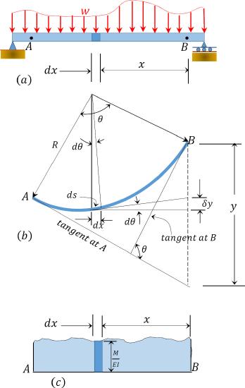
Fig.7.8. Deflected beam.
Substituting equation 7.14 into equation 7.8 suggests the following:
dθ=MEIds
Since ds is infinitesimal because of the small lateral deflection of the beam that is allowed in engineering, it can be replaced by its horizontal projection dx. Thus,
dθ=MEIdx
The angle θ between the tangents at A and B can thus be obtained by summing up the subtended angles by the infinitesimal length lying between these points. Thus,
∫BAdθ=∫BAMEIdxOrθB/A=θB−θA=∫BAMEIdx
Equation 7.17 is referred to as the first moment-area theorem. The first moment-area theorem states that the total change in slope between A and B is equal to the area of the bending moment diagram between these two points divided by the flexural rigidity EI.
Second Moment-Area Theorem
Referring again to Figure 7.8, it is required to determine the tangential deviation of point B with respect to point A, which is the vertical distance of point B from the tangent drawn to the elastic curve at point A. To do so, first calculate the contribution δΔ of the element of length dL to the vertical distance. According to geometry,
δy=xdθ
Substituting dθ from equation 7.15 to equation 7.18 suggests the following:
δy=MxEIdx
Hence,
y=∫BAMxEIdx
Equation 7.20 is referred to as the second moment area theorem. The second moment-area theorem states that the vertical distance of point B on an elastic curve from the tangent to the curve at point A is equal to the moment with respect to the vertical through B of the area of the bending moment diagram between A and B, divided by the flexural rigidity, EI.
Sign Conventions
The sign conventions for moment-area theorems are as follows:
(1)The tangential deviation of a point B, with respect to a tangent drawn at the elastic curve at a point A, is positive if B lies above the drawn tangent at A and negative if it lies below the tangent (see Figure 7.9).
(2)The slope at a point B, with respect to a tangent drawn at a point A in an elastic curve, is positive if the tangent drawn at B rotates in a counterclockwise direction with respect to the tangent at A and negative if it rotates in a clockwise direction (see Figure 7.9).
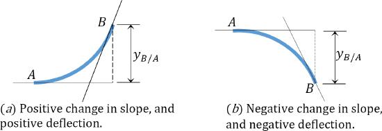
Fig.7.9. Sign convention representation.
Procedure for Analysis by Moment-Area Method
•Sketch the free-body diagram of the beam.
•Draw the M/EI diagram of the beam. This will look like the conventional bending moment diagram of the beam if the beam is prismatic (i.e. of the same cross section for its entire length).
•To determine the slope at any point, find the angle between a tangent passing the point and a tangent passing through another point on the deflected curve, divide the M/EI diagram into simple geometric shapes, and then apply the first moment-area theorem. To determine the deflection or a tangential deviation of any point along the beam, apply the second moment-area theorem.
•In cases where the configuration of the M/EI diagram is such that it cannot be divided into simple shapes with known areas and centroids, it is preferable to draw the M/EI diagram by parts. This entails introducing a fixed support at any convenient point along the beam and drawing the M/EI diagram for each of the applied loads, including the support reactions, prior to the application of any of the theorems to determine what is required.
Table 7.1. Areas and centroids of geometric shapes.
| Geometric Shape | Area | Centroid | ||
| C1 | C2 | |||
| Rectangle | 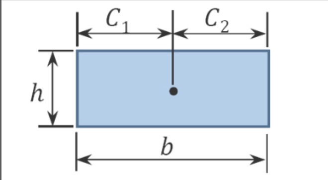 |
bh | b2 | b2 |
| Triangle | 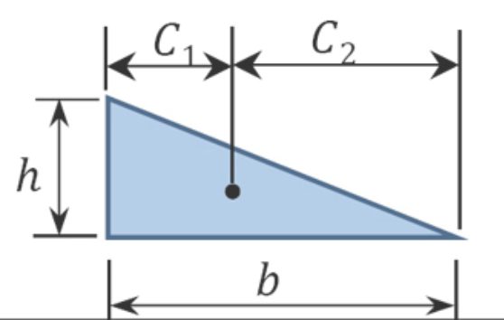 |
bh2 | b3 | 2b3 |
| Parabolic Spandrel | 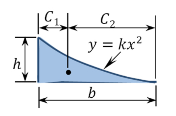 |
bh3 | b4 | 3b4 |
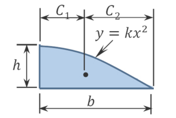 |
2bh3 | 3b8 | 5b8 | |
| Cubic Spandrel | 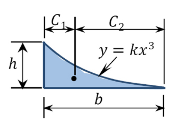 |
bh4 | b5 | 4b5 |
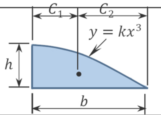 |
3bh4 | 2b5 | 3b5 | |
| General Spandrel | 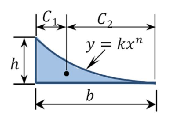 |
bhn+1 | bn+2 | b(n+1)n+2 |
Example 7.7
A cantilever beam shown in Figure 7.10a is subjected to a concentrated moment at its free end. Using the moment-area method, determine the slope at the free end of the beam and the deflection at the free end of the beam. EI = constant.
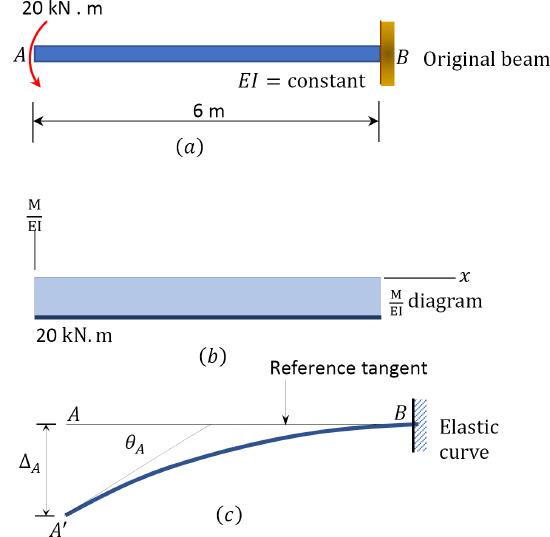
Fig.7.10. Cantilever beam.
Solution
(M/EI) diagram. First, draw the bending moment diagram for the beam and divide it by the flexural rigidity, EI, to obtain the MEI diagram shown in Figure 7.10b.
Slope at A. The slope at the free end is equal to the area of the MEI diagram between A and B, according to the first moment-area theorem. Using this theorem and referring to the MEI diagram suggests the following:
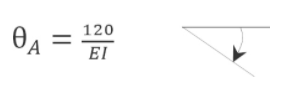
θA=−(1EI)(6)(20)=−120EI
Deflection at A. The deflection at the free end of the beam is equal to the moment with respect to the vertical through A of the area of the MEI diagram between A and B, according to the second moment-area theorem. Using this theorem and referring to Figure 7.10b and Figure 7.10c suggests the following:
ΔA=−(1EI)(6)(20)(3)=−360EIΔA=360EI↓
Example 7.8
A propped cantilever beam carries a uniformly distributed load of 4 kips/ft over its entire length, as shown in Figure 7.11a. Using the moment-area method, determine the slope at A and the deflection at A.
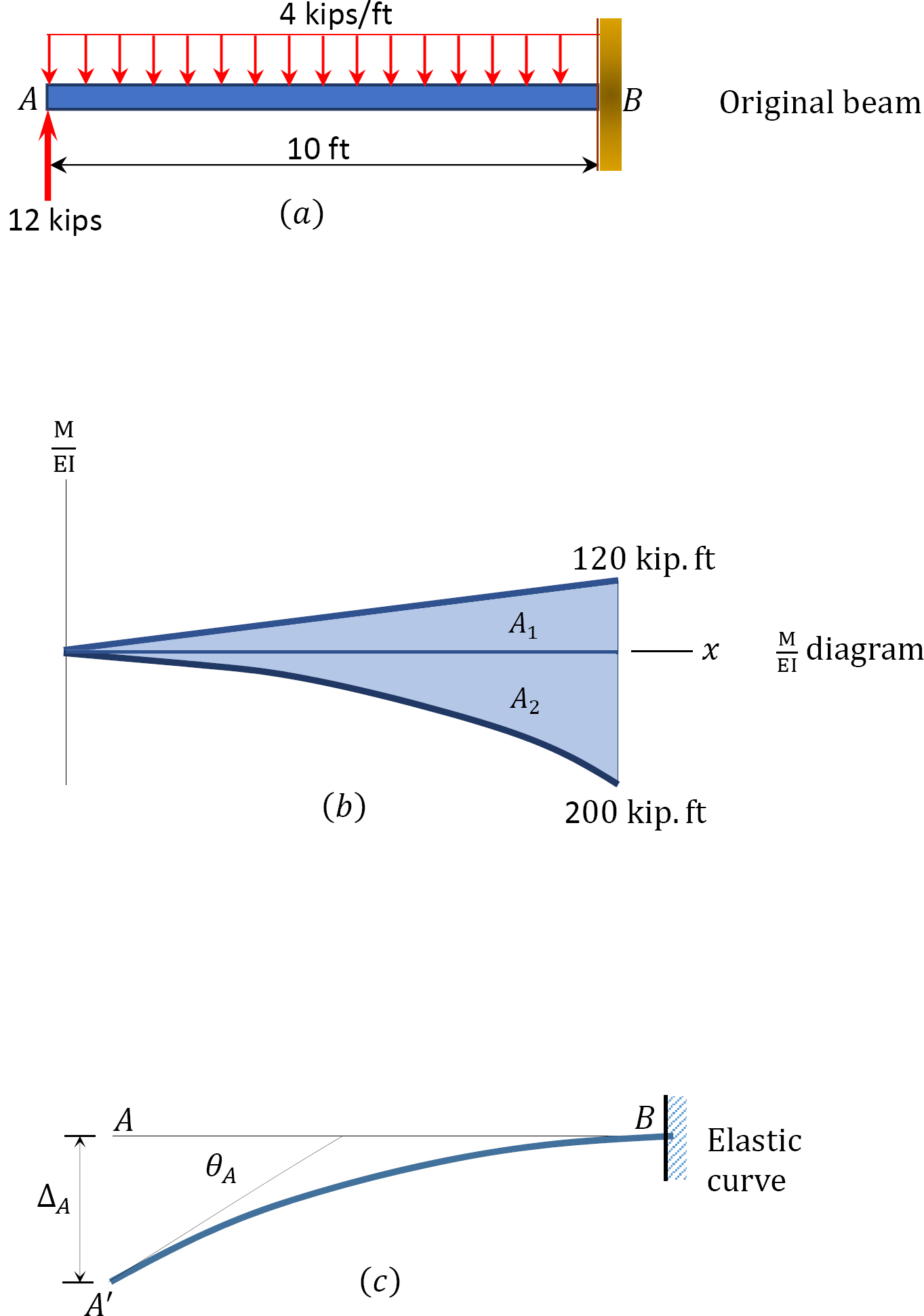
Fig.7.11. Propped cantilever beam.
Solution
(M/EI) diagram. First, draw the bending moment diagram for the beam and divide it by the flexural rigidity, EI, to obtain the MEI diagram shown in Figure 7.11b.
Slope at A. The slope at the free end is equal to the area of the MEI diagram between A and B. The area between these two points is indicated as A1 and A2 in Figure 7.11b. Use Table 7.1 to find the computation of A2, whose arc is parabolic, and the location of its centroid. Noting from the table that A=13bh and applying the first moment-area theorem suggests the following:
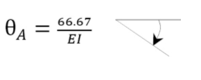
θA=A1−A2=(1EI)(12)(10)(120)−(1EI)(10×2003)=−66.67EI
Deflection at A. The deflection at A is equal to the moment of area of the MEI diagram between A and B about A. Thus, using the second moment-area theorem and referring to Figure 7.11b and Figure 7.11c suggests the following:
ΔA=A1(L3)−A2(3L4)=(1EI)(12)(10)(120)(2×10³)−(1EI)(10×2003)(3×10⁴)=−1000EIΔA=1000EI↓
Example 7.9
A simply supported timber beam with a length of 8 ft will carry a distributed floor load of 500 lb/ft over its entire length, as shown Figure 7.12a. Using the moment area theorem, determine the slope at end B and the maximum deflection.
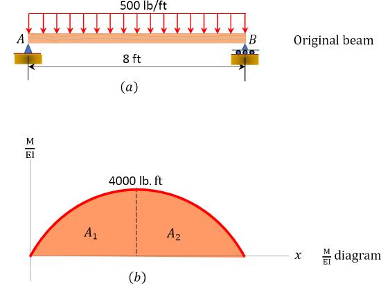
Fig.7.12. Simply supported timber beam.
Solution
(M/EI) diagram. First, draw the bending moment diagram for the beam, and divide it by the flexural rigidity, EI, to obtain the MEI diagram shown in Figure 7.12b.
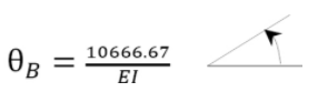
Slope at B. The slope at B is equal to the area of the MEI diagram between B and C. The area between these two points is indicated as A2 in Figure 7.12b. Applying the first moment-area theorem suggests the following:
θB=A2=(1EI)(2bh3)=(1EI)(2(4)(4000)3)=10666.67EI
Maximum deflection. The maximum deflection occurs at the center of the beam (point C). It is equal to the moment of the area of the MEI diagram between B and C about B. Thus,
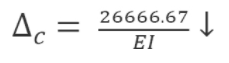
Δc=A2(5b8)=(1EI)(2(4)(4000)3)(5(4)8)=26666.67EI
Example 7.10
A prismatic timber beam is subjected to two concentrated loads of equal magnitude, as shown in Figure 7.13a. Using the moment-area method, determine the slope at A and the deflection at point C.
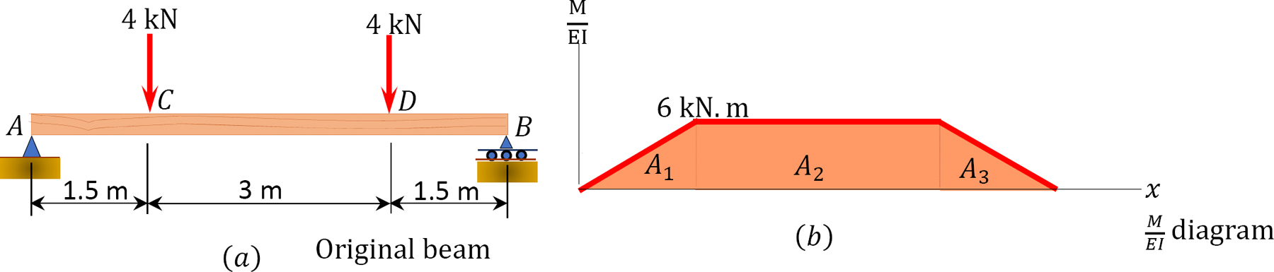
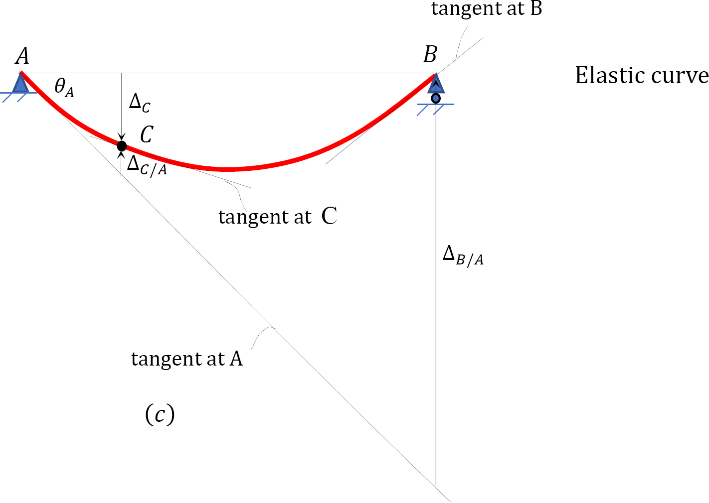
Fig.7.13. Prismatic timber beam.
Solution
(M/EI) diagram. First, draw the bending moment diagram for the beam and divide it by the flexural rigidity, EI, to obtain the MEI diagram shown in Figure 7.13b.
Slope at A. The deflection and the rotation of the beam are small since they occur within the elastic limit. Thus, the slope at support A can be computed using the small angle theorem, as follows:
θA=ΔB/AL=ΔB/A6
To determine the tangential deviation of B from A, apply the second moment-area theorem. According to the theorem, it is equal to the moment of the area of the MEI diagram between A and B about B. Thus,
ΔB/A=A1(1.5+3+13×1.5)+A2(1.5+1.5)+A3(23×1.5)ΔB/A=1EI[12(1.5)(6)(23×1.5)+(3)(6)(1.5+1.5)+12(1.5)(6)(1.5+3+13×1.5)]ΔB/A=81EI
Thus, the slope at A is
θA=ΔB/AL=816EI=13.5EIθA=13.5EI
Deflection at C. The deflection at C can be obtained by proportion.
ΔB/A6=Δc+ΔC/A1.5Δc=(1.5)(ΔB/A)6−ΔC/A
Similarly, the tangential deviation of C from A can be determined as the moment of the area of the MEI diagram between A and C about C.
ΔC/A=1EI[12(1.5)(6)(23×1.5)]=92EI
Therefore, the deflection at C is
Δc=(1.5)(81)6EI−92EI=15.75EIΔc=15.75EI