8.1: Virtual Work Method

The virtual work method, also referred to as the method of virtual force or unit-load method, uses the law of conservation of energy to obtain the deflection and slope at a point in a structure. This method was developed in 1717 by John Bernoulli. To illustrate the principle of virtual work, consider the deformable body shown in Figure 8.1. First, applying a virtual or fictitious unit load \(P_{V}=1\) at a point \(Q\), where the deflection parallel to the applied load is desired, will create an internal virtual or imaginary load \(f\) and will cause point \(Q\) to displace by a certain small amount. Then, placing the real external loads \(P_{1}\), \(P_{2}\), and \(M\) on the same body will cause an internal deformation, \(dS\), and an external deflection of point \(Q\) to \(Q^{\prime}\) by an amount \(\Delta\).

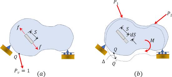
\(Fig. 8.1\). Deformable body.

Upon placement of the real load, the point of application of the virtual load also displaces by \(\Delta\), and the applied unit load performs work by traveling the distance \(\Delta\). The work done by the virtual forces are as follows:

External work done by the unit load \(P_{V}\)

\[\begin{array}{l}
=P_{v} \times \text { Displacement } \\
=1 \times \Delta
\end{array}\]

Internal work done by the virtual load \(f\)

\[=f \times d S\]

Applying the principle of conservation of energy by equating equation 8.1 and equation 8.2 suggests the following:

External work done = Internal work done

where

• \(P_{V} = 1\) = external virtual unit load.
• \(f\) = internal virtual load.
• \(\Delta\) = external displacement caused by real loads.
• \(dS\) = internal deformation caused by real loads.

Similarly, to obtain the slope at a point on a structure, apply a unit virtual moment \(M_{V}\) at the specified point where the slope is desired, and apply the following equation derived via the principle of conservation of energy:

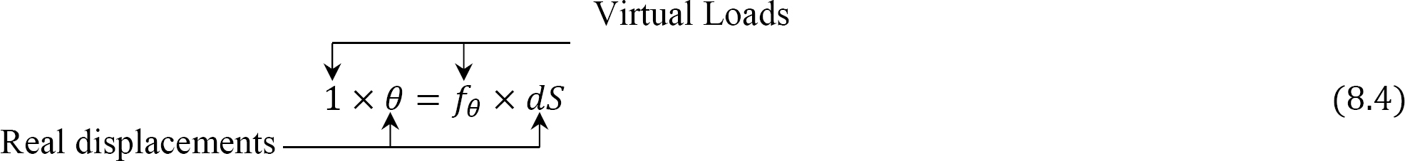
where

• \(M_{V} = 1\) = external virtual unit moment.
• \(f\) = internal virtual load.
• \(\theta\) = external rotational displacement caused by real loads.
• \(dS\) = internal deformation caused by real loads.

Virtual Work Formulation for the Deflection and Slope of Beams and Frames

To develop the equations for the computation of deflection of beams and frames using the virtual work principles, consider the beam loaded as shown in Figure 8.2a. The deflection at point C due to the applied external loads is required. First, removing the loads \(P\) and \(W\) and applying a virtual unit load \(P_{V} = 1\) will cause elementary forces and deformations to develop in the bar, and a small deflection to occur at \(C\), as follows:

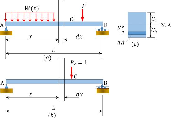
\(Fig. 8.2\). Loaded beam.

The stress acting on the differential cross-sectional area \(dA\) at a distance x from the left-end support due to a virtual unit load is as follows:

\[\sigma^{\prime}=\frac{m y}{I}\]

where \(m\) is the internal virtual moment at the section at a distance xe from the left-end support due to the virtual unit load and \(I\) is the moment of inertia of the section.

The force acting on the differential area due to the virtual unit load is written as follows:

\[f=\sigma^{\prime} d A=\left(\frac{m y}{I}\right) d A\]

The stress due to the external loads \(P_{1}\) and \(P_{2}\) on the beam is written as follows:

\[\sigma=\frac{M y}{I}\]

The deformation of a differential beam length \(dx\) at a distance \(x\) from the left-end support is as follows:

\[\delta=\varepsilon d x=\left(\frac{\sigma}{E}\right) d x=\left(\frac{M y}{E I}\right) d x\]

The work done by the force \(f\) acting on the differential area due to the deformation of the differential beam length \(dx\) is as follows:

\[\begin{array}{c}
d W=f \delta=\left(\frac{m y}{I}\right) d A \times\left(\frac{M y}{E I}\right) d x \\
=\left(\frac{M m y^{2}}{E I^{2}}\right) d A d x
\end{array}\]

The internal work done by the total force in the entire cross-sectional area of the beam due to the applied virtual unit load when the differential length of the beam \(dx\) deforms by \(\delta\) can be obtained by integrating with respect to \(dA\), as follows:

\[\begin{aligned}
\int_{A} d W &=\left[\int_{A_{1}}^{A_{n}}\left(\frac{M m y^{2}}{E I}\right) d A\right] d x \\
W_{i} &=\left(\frac{M m}{E I^{2}} \int y^{2} d A\right) d x \\
&=\left[\left(\frac{M m}{E I^{2}}\right) I\right] d x \\
&=\left(\frac{M m}{E I}\right) d x
\end{aligned}\]

The internal work done \(W_{i}\) in the entire length of the beam due to the applied virtual unit load can now be obtained by integrating with respect to \(dx\), which is written as follows:

\[W_{i}=\int_{0}^{L}\left(\frac{M m}{E I}\right) d x\]

The external work done \(W_{e}\) by the virtual unit load due to the deflection \(\Delta\) at point \(C\) of the beam caused by the external loads is as follows:

\[W_{e}=1 \times \Delta\]

The principle of conservation of energy is applied to obtain the expression for the computation of the deflection at any point in a beam or frame, which is written as follows:

\[\begin{aligned}
W_{e} &=W_{i} \\
1 \times \Delta &=\int_{0}^{L}\left(\frac{M m}{E I}\right) d x \\
\Delta &=\int_{0}^{L}\left(\frac{M m}{E I}\right) d x
\end{aligned}\]

where

• \(1\) = external virtual or imaginary unit load on the beam or frame in the direction of the required deflection \(\Delta\).
• \(\Delta\) = external displacement at the specified point on a beam or frame caused by the real loads.
• \(M\) = internal moment in the beam or frame caused by the real load, expressed in terms of the horizontal distance x.
• \(m\) = internal virtual moment in the beam or frame caused by the external virtual unit load, expressed with respect to the horizontal distance x.
• \(E\) = modulus of elasticity of the material of the beam or frame.
• \(I\) = moment of inertia of the cross-sectional area of the beam or frame about its neutral axis.

Similarly, the following expression can be obtained for the computation of the slope at a point in a beam or frame:

\[\theta=\int_{0}^{L} \frac{M m_{\theta}}{E I} d x\]

where

\(\theta\) = slope or tangent rotation at a point on a beam or frame.

\(m_{\theta}\) = internal virtual moment in the beam or frame, expressed with respect to the horizontal distance \(x\), caused by the external virtual unit moment applied at the point where the rotation is required.

Procedure for Determination of Deflection in Beams and Frames by the Virtual Work Method

• Determine the support reactions in the real system using the equations of static equilibrium.
• Write an expression for the moment in the real structure as a function of the horizontal distance \(x\). The number of the equations will depend on the number of regions of the beam due to discontinuous loading.
• Create a virtual system by removing all the loads acting on the beam and applying a unit load or a unit moment at the point where the deflection or slope is desired.
• Write the moment expression for the virtual system in terms of the distance \(x\).
• Substitute the moment expressions into equation 8.1 and integrate to obtain the value of deflection or slope at the point considered.

Virtual Work Formulation for the Deflection of Trusses

Consider the truss shown in Figure 8.3 for the development of the virtual work expression for the determination of the deflection of trusses. The truss is subjected to the loads \(P_{1}\), \(P_{2}\), and \(P_{3}\), and the vertical deflection \(\Delta\) at joint \(F\) is desired. First, remove the loads \(P_{1}\), \(P_{2}\), and \(P_{3}\), and apply a vertical virtual unit load \(P_{v} = 1\) at joint \(F\), as shown in Figure 8.3b. The virtual unit load will cause the virtual internal axial load \(n_{i}\) to act on each member of the truss. Applying the forces \(P_{1}\), \(P_{2}\), and \(P_{3}\) will cause the deflection \(\Delta\) at joint \(F\) and the internal deformation \(\delta L_{i}\) in each member of the truss.

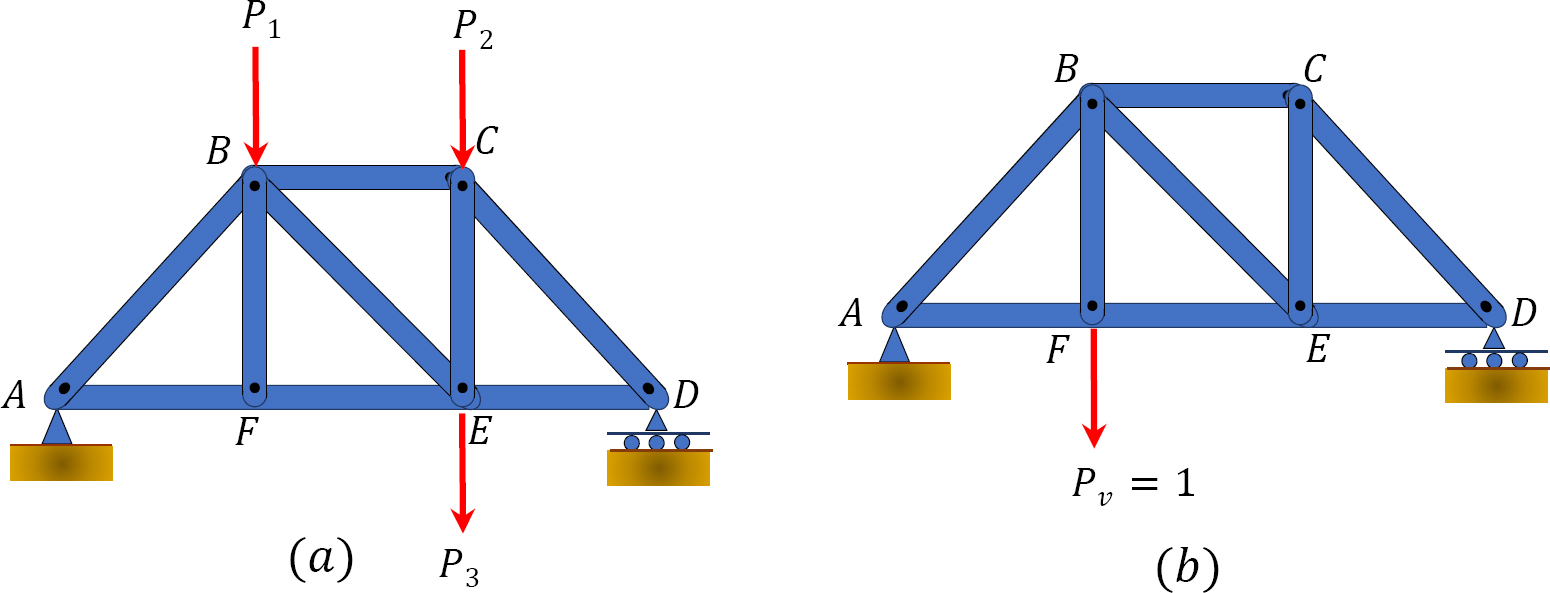
\(Fig. 8.3\). Sample truss.

Using the law of conservation of energy, the work by the virtual unit load at joint \(F\) and the virtual internal axial loads on the members of the truss can be written as follows:

External work = internal work

\[1 \times \Delta=\sum_{i=1}^{n} n_{i}\left(\delta L_{i}\right)\]

But, for a member with length \(L_{i}\), area \(A_{i}\), and material Young’s modulus \(E_{i}\), the deformation is written as follows:

\[\delta L_{i}=\frac{N_{i} L_{i}}{A_{i} E_{i}}\]

Thus, the virtual work expression for the deflection of a truss can be written as follows:

\[\Delta=\sum_{i=1}^{n} n_{i}\left(\frac{N_{i} L_{i}}{A_{i} E_{i}}\right)\]

where

1 = external vertical virtual unit load applied at joint \(F\).

\(n\) = internal axial virtual force in each truss member due to the virtual unit load, \(P_{v} = 1\).

\(N\) = axial force in each truss member due to the real loads \(P_{1}\), \(P_{2}\), and \(P_{3}\).

\(\Delta\) = external joint displacement caused by the real loads.

\(\delta L\) = deformation of each truss member caused by the real loads.

Procedure for Determination of Deflection in Trusses by the Virtual Work Method

• Determine the support reactions in the real system with the applied loads using the equations of equilibrium.
• Determine the internal forces \(N\) in truss members caused by the external loads on the real system.
• Remove all the external loads on the real system and apply a virtual unit load on the joint in the truss in the direction of required deflection.
• Determine the internal virtual forces \(n\) in the members of the truss caused by the external virtual unit load placed in the joint where the deflection is desired.
• Calculate the deflection \(\Delta\) in the joint of the truss caused by the real loads using equation 8.17.

Example 8.1

Using the virtual work method, determine the deflection and the slope at a point \(B\) of the cantilever beam shown in Figure 8.4a. \(E=29 \times 10^{3} \mathrm{ksi}, I=600 \mathrm{in}^{4}\).

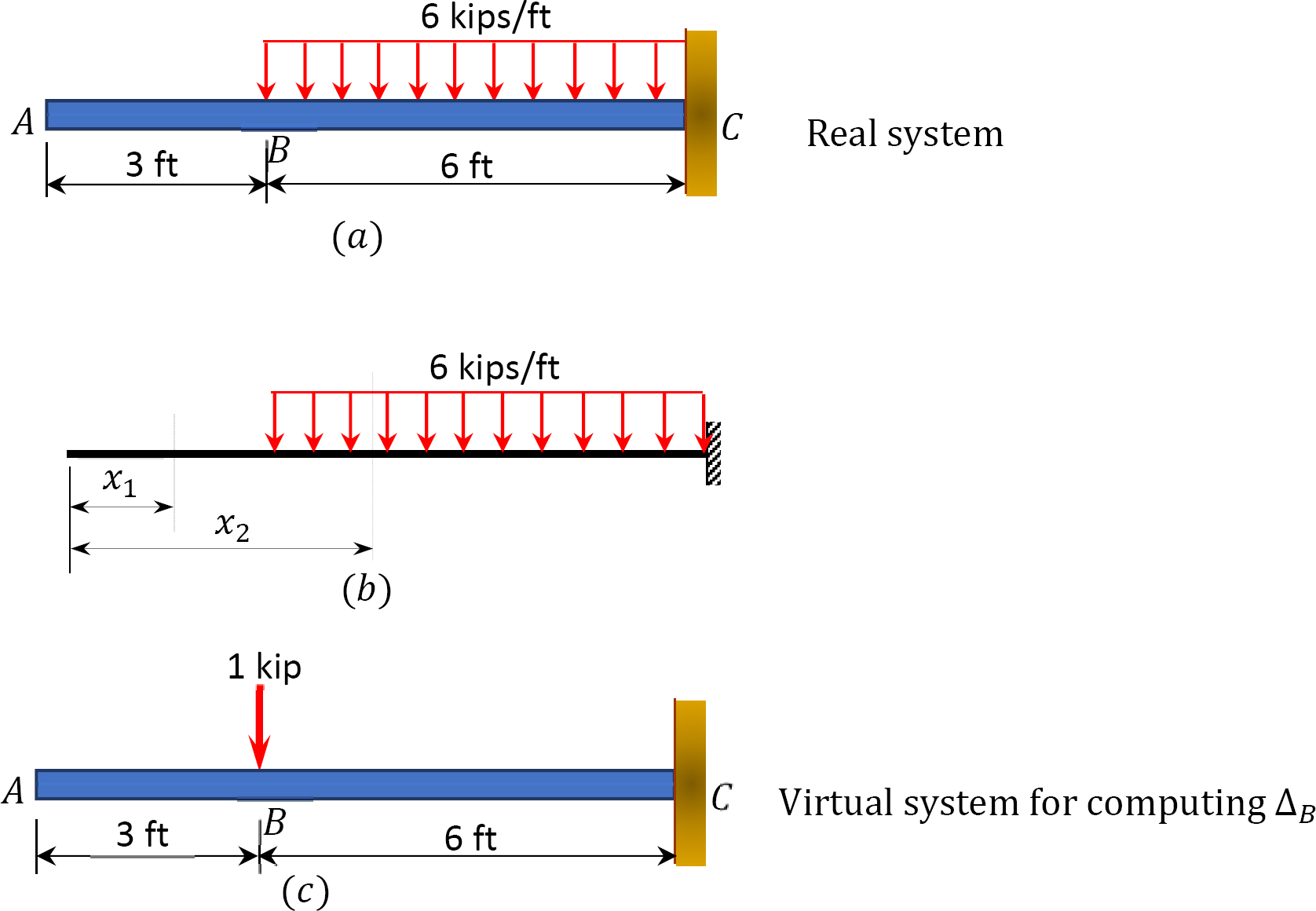
\(Fig. 8.4\). Cantilever beam.

Solution

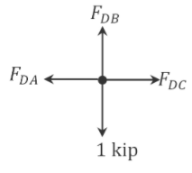
Real and virtual systems. The real and virtual systems are shown in Figure 8.4a, Figure 8.4c, and Figure 8.4e, respectively. Notice that the real system consists of the external loading carried by the beam, as specified in the problem. The virtual system consists of a unit 1-k load applied at \(B\), where the deflection is required, and 1-k-ft moment applied at the same point where the slope is determined. The bending moments at each portion of the beam, with respect to the horizontal axis, are presented in Table 8.1. Notice that the origin of the horizontal distance, \(x\), for both the real and virtual system is at the free end, as shown in Figure 8.4b, Figure 8.4d, and Figure 8.4f.

\(Table 8.1\). Bending moments at portions of the beam.

Portion	X-Coordinate		Deflection		Slope
	Origin	Limit (ft)	M	M	M	\(m_{\theta}\)
AB	A	0-3	0	0	0	0
BC	A	3-9	-3(x-3)^2	1(x-3)	-3(x-3)^2	-1

Deflection at \(B\). The deflection at the free end of the beam is determined by using equation 8.1, as follows:

\(\begin{array}{l}
1 \mathrm{kip} . \Delta_{B}=\int_{0}^{L} \frac{m M}{E I} d x=\int_{0}^{3} \frac{(0)(0) d x}{E I}+\int_{3}^{9} \frac{-3(x-3)^{2}(x-3) d x}{E I} \\
1 \mathrm{kip.} \Delta_{B}=\frac{-972 \mathrm{k} \cdot \mathrm{ft}^{3}}{E I}
\end{array}\)

Therefore,

\(\begin{aligned}
\Delta_{B} &=\frac{-972 \mathrm{k} \cdot \mathrm{ft}^{3}(12)^{3} \mathrm{in}^{3} / \mathrm{ft}^{3}}{\left(29 \times 10^{3} \mathrm{k} / \mathrm{in}^{2}\right)\left(600 \mathrm{in}^{4}\right)} \\
&=-0.097 \mathrm{in.} \quad \Delta_{B}=0.097 \mathrm{in} . \uparrow
\end{aligned}\)

Slope at \(B\). The slope at the free end of the beam is determined by using equation 8.2, as follows:

\(\begin{array}{l}
(1 \mathrm{kN}. \mathrm{m}). \theta_{B}=\int_{0}^{L} \frac{\mathrm{m}_{\theta} M}{E I} d x=\int_{0}^{3} \frac{(0)(0) d x}{E I}+\int_{3}^{9} \frac{-3(x-3)^{2}(-1) d x}{E I} \\
(1 \mathrm{k.ft}). \theta_{B}=\frac{216 \mathrm{k}^{2} . \mathrm{ft}^{3}}{E I}=\frac{216 \mathrm{k}^{2} \cdot \mathrm{ft}^{3}}{\left(29 \times 10^{3} \mathrm{k} / \mathrm{in}^{2}\right)\left(600 \mathrm{in}^{4}\right)}
\end{array}\)

Therefore,

\(\theta_{B}=\frac{216 \mathrm{k} \cdot \mathrm{ft}^{2}}{\left(29 \times 10^{3} \mathrm{k} / \mathrm{in}^{2}\right)\left(600 \mathrm{in}^{4}\right)}=\frac{216(12)^{2}}{\left(29 \times 10^{3} \mathrm{k} / \mathrm{in}^{2}\right)\left(600 \mathrm{in}^{4}\right)}=0.0018 \mathrm{rad}\)

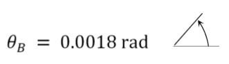
Example 8.2

Using the virtual work method, determine the deflection at \(B\) and the slope at \(C\) for the simply supported beam subjected to a concentrated load, as shown in Figure 8.5a. \(EI\) = constant. \(E=29 \times 10^{3} \mathrm{ksi} . I=24 \mathrm{in}^{4}\).

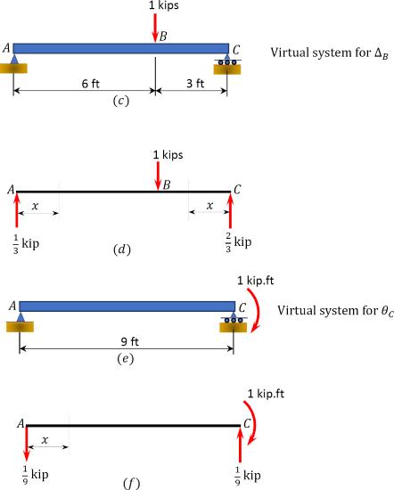
\(Fig. 8.5\). Simply supported beam.

Solution

Real and virtual systems. The real and virtual systems are shown in Figure 8.5a, Figure 8.5c, and Figure 8.5e, respectively. The bending moments at each portion of the beam, with respect to the horizontal axis, are presented in Table 8.2. The origin of the horizontal distances for both the real and virtual system are shown in Figure 8.5b, Figure 8.5d, and Figure 8.5f.

\(Table 8.2\). Bending moments at portions of the beam.

Portion	x Coordinate		Deflection		Slope
	Origin	Limit (ft)	M	m	M	\(m_{\theta}\)
AB	A	0-6	4x	\(\frac{x}{3}\)	4x	\(-\frac{x}{9}\)
CB	C	0-3	8x	\(\frac{2x}{3}\)	8x	\(\frac{x}{9}-1\)

Deflection at \(B\). The deflection at \(B\) can be determined by using equation 8.1, as follows:

\(\begin{array}{l}
1 \mathrm{kip} . \Delta_{B}=\int_{0}^{L} \frac{m M}{E I} d x=\int_{0}^{6} \frac{(4 x)\left(\frac{x}{3}\right) d x}{E I}+\int_{0}^{3(8 x)\left(\frac{2 x}{3}\right) d x}{E I} \\
1 \text { kip. } \Delta_{B}=\frac{144 \mathrm{k}, \mathrm{ft}^{3}}{F I}
\end{array}\)

Therefore,

\(\Delta_{B}=\frac{144 \mathrm{k} \cdot \mathrm{ft}^{3}(12)^{3} \mathrm{in}^{3} / \mathrm{ft}^{3}}{\left(29 \times 10^{3} \mathrm{k} / \mathrm{in}^{2}\right)\left(24 \mathrm{in}^{4}\right)}=0.36 \text { in } \quad \Delta_{B}=0.36 \mathrm{in.} \downarrow\)

The positive value indicates deflection in the direction of the applied virtual load.

Slope at \(C\). The slope at \(C\) can be determined by using equation 8.2, as follows:

\(\begin{array}{l}
(1 \mathrm{k} . \mathrm{ft}). \theta_{C}=\int_{0}^{L} \frac{\mathrm{m}_{\theta} M}{E I} d x=\int_{0}^{6} \frac{(4 x)\left(-\frac{x}{9}\right) d x}{E I}+\int_{0}^{3} \frac{(8 x)\left(\frac{x}{9}-1\right) d x}{E I} \\
(1 \mathrm{k.ft}). \theta_{C}=-\frac{60 \mathrm{k}^{2} \cdot \mathrm{ft}^{3}}{E I}=-\frac{60 \mathrm{k}^{2} \cdot \mathrm{ft}^{3}}{\left(29 \times 10^{3} \mathrm{k} / \mathrm{in}^{2}\right)\left(24 \mathrm{in}^{4}\right)}
\end{array}\)

Therefore,

\(\begin{aligned}
\theta_{C} &=-\frac{60 \mathrm{k} . \mathrm{ft}^{2}}{\left(29 \times \frac{10^{3} \mathrm{k}}{\mathrm{in}^{2}}\right)\left(24 \mathrm{in}^{4}\right)}=-\frac{60(12)^{2}}{\left(29 \times 10^{3} \mathrm{k} / \mathrm{in}^{2}\right)\left(24 \mathrm{in}^{4}\right)} \\
&=-0.012 \mathrm{rad}
\end{aligned}\)

Example 8.3

Using the virtual work method, determine the deflection at \(B\) and the slope at \(D\) for the compound beam shown in Figure 8.6a. \(E=200 \text { GPa and } I=250 \times 10^{6} \mathrm{~mm}^{4}\).

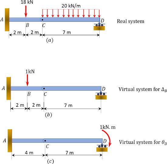
\(Fig. 8.6\). Compound beam.

Solution

Real and virtual systems. The real and virtual systems are shown in Figure 8.6a, Figure 8.6b, and Figure 8.6c, respectively. The bending moment at each portion of the beam, with respect to the horizontal axis, are presented in Table 8.3.

\(Table 8.3\). Bending moments at portions of the beam.

Portion	X-Coordinate		Deflection		Slope
	Origin	Limit (ft)	M	m	M	\(m_{\theta}\)
DC	D	0-7	\(70x-10x^2\)	0	\(70x-10x^2\)	\(\frac{x}{7}-1\)
CB	C	0-2	\(-70x\)	0	\(-70x\)	\(\frac{x}{7}\)
BA	C	2-4	\(-70x-18(x-2)\)	\(-x\)	\(-70x-18(x-2)\)	\(\frac{x}{7}\)

Deflection at \(B\). The deflection at \(B\) can be determined using equation 8.1, as follows:

\(\begin{aligned}
1 \mathrm{kN.} \Delta_{B} &=\int_{0}^{L} \frac{m M}{E I} d x=\int_{0}^{7} \frac{(0)\left(70 x-10 x^{2}\right) d x}{E I}+\int_{0}^{2} \frac{(0)(-70 x) d x}{E I}+\int_{2}^{4} \frac{(-x)[-70 x-18(x-2)] d x}{E I} \\
1 \mathrm{kN} . \Delta_{B} &=\frac{1426.67 \mathrm{kN}^{2} \cdot \mathrm{m}^{3}}{E I}
\end{aligned}\)

Therefore,

\(\Delta_{B}=\frac{1426.67 \mathrm{kN} \cdot \mathrm{m}^{3}}{\left(200 \times 10^{6} \mathrm{kN} / \mathrm{m}^{2}\right)\left(250 \times 10^{6} \mathrm{~mm}^{4}\right)\left(10^{-12} \mathrm{~m}^{4} / \mathrm{mm}^{4}\right)}=0.0285 \mathrm{~m} \quad \Delta_{B}=28.5 \mathrm{~mm} \downarrow\)

Slope at \(D\). The slope at \(D\) can be determined using equation 8.2, as follows:

\(\begin{array}{l}
(1 \mathrm{kN} \cdot \mathrm{m}) \cdot \theta_{D}=\int_{0}^{L} \frac{\mathrm{m}_{\theta} M}{E I} d x=\int_{0}^{7} \frac{\left(\frac{x}{7}-1\right)\left(70 x-10 x^{2}\right) d x}{E I}+\int_{0}^{2} \frac{\left(\frac{x}{7}\right)(-70 x) d x}{E I}+\int_{2}^{4} \frac{\left(\frac{x}{7}\right)[-70 x-18(x-2)] d x}{E I} \\
(1 \mathrm{kN} \cdot \mathrm{m}) \cdot \theta_{D}=-\frac{516.31 \mathrm{kN}^{2} \cdot \mathrm{m}^{3}}{E I}
\end{array}\)

Therefore,

\(\theta_{D}=\frac{-516.31 \mathrm{kN} \cdot \mathrm{m}^{3}}{\left(200 \times 10^{6} \mathrm{kN} / \mathrm{m}^{2}\right)\left(250 \times 10^{6} \mathrm{~mm}^{4}\right)\left(10^{-12} \mathrm{~m}^{4} / \mathrm{mm}^{4}\right)}=-0.0103 \mathrm{rad}\)

The negative sign indicates that the rotation at point \(D\) is in the direction opposite to the applied virtual moment.

Example 8.4

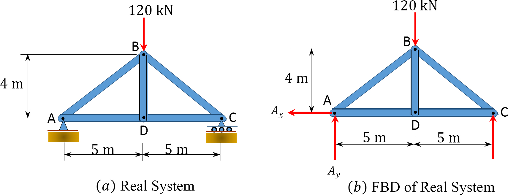
Using the virtual work method, determine the slope at joint \(A\) of the frame shown in Figure 8.7a. \(E=29 \times 10^{3} \mathrm{ksi} \text { and } E I=700 \mathrm{in}^{4}\).

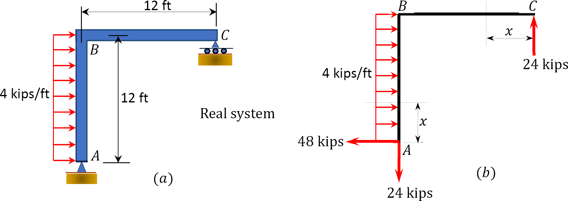
\(Fig. 8.7\). Frame.

Solution

Real and virtual systems. The real and virtual systems are shown in Figure 8.7a and Figure 8.7c, respectively. The bending moment at each segment of the beam and column of the frame are presented in Table 8.4, and their origins are shown in Figure 8.7b and Figure 8.7d.

\(Table 8.4\). Bending moments at portions of the beam.

Portion	X-Coordinate		Deflection
	Origin	Limit	M	m
AB	0	0-12	\(48x-2x^2\)	1
CB	0	0-12	\(24x\)	\(\frac{x}{12}\)

Slope at \(A\). The slope at \(A\) can be determined by using equation 8.2, as follows:

\(\begin{aligned}
(1 \mathrm{k} \cdot \mathrm{ft}) \cdot \theta_{A} &=\int_{0}^{L} \frac{\mathrm{m}_{\theta} M}{E I} d x=\int_{0}^{12} \frac{(1)\left(48 x-2 x^{2}\right) d x}{E I}+\int_{0}^{12} \frac{(24 x)\left(\frac{x}{12}\right) d x}{E T} \\
(1 \mathrm{k.ft}) \cdot \theta_{A} &=\frac{3456 \mathrm{k}^{2} \cdot \mathrm{ft}^{3}}{E I}
\end{aligned}\)

Therefore,

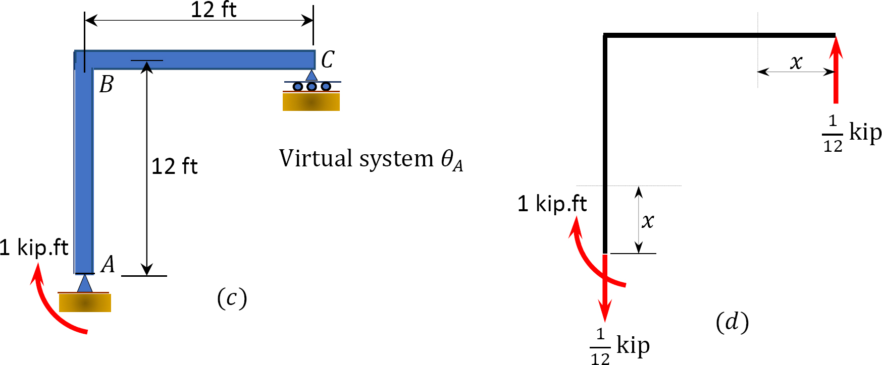
\(\theta_{A}=\frac{3456 \mathrm{k} . \mathrm{ft}^{2}}{\left(29 \times 10^{3} \mathrm{k} / \mathrm{in}^{2}\right)\left(700 \mathrm{in}^{4}\right)}=\frac{3456(12)^{2}}{\left(29 \times 10^{3} \mathrm{k} / \mathrm{in}^{2}\right)\left(700 \mathrm{in}^{4}\right)}=0.0245 \mathrm{rad}\)

Example 8.5

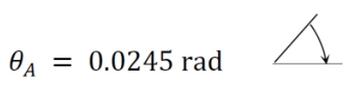
Using the virtual work method, determine the vertical deflection at \(A\) of the frame shown in Figure 8.8a. \(E=200 \text { GPa and } I=250 \times 10^{6} \mathrm{~mm}^{4}\).

\(Fig. 8.8\). Frame.

Solution

Real and virtual systems. The real and virtual systems are shown in Figure 8.8a and Figure 8.8c, respectively. The bending moment at each segment of the beam and column of the frame are presented in Table 8.5, and their origins are shown in Figure 8.8b and Figure 8.8d.

\(Table 8.5\). Bending moments at portions of the beam.

Portion	X-Coordinate		Deflection
	Origin	Limit	M	m
AB	A	0-4	0	-x
BC	A	4-8	\(-16(x-4)\)	-x
CE	C	0-10	-64	-8

Deflection at \(A\). The deflection at \(A\) can be determined by using equation 8.1, as follows:

\(\begin{array}{l}
1 \mathrm{kN} . \Delta_{A}=\int_{0}^{L} \frac{m M}{E I} d x=\int_{0}^{4} \frac{(0)(-x) d x}{E I}+\int_{4}^{8} \frac{(-16(x-4))(-x) d x}{E I}+\int_{0}^{10} \frac{(-8)(-64) d x}{E I} \\
\mathrm{kN} . \Delta_{A}=\frac{853.33 \mathrm{kN}^{2} \cdot \mathrm{m}^{3}}{E I}
\end{array}\)

Therefore,

\(\Delta_{A}=\frac{853.33 \mathrm{kN} \cdot \mathrm{m}^{3}}{\left(200 \times 10^{6} \mathrm{kN} / \mathrm{m}^{2}\right)\left(250 \times 10^{6} \mathrm{~mm}^{4}\right)\left(10^{-12} \mathrm{~m}^{4} / \mathrm{mm}^{4}\right)}=0.017 \mathrm{~m} \quad \Delta_{A}=17 \mathrm{~mm} \downarrow\)

Example 8.6

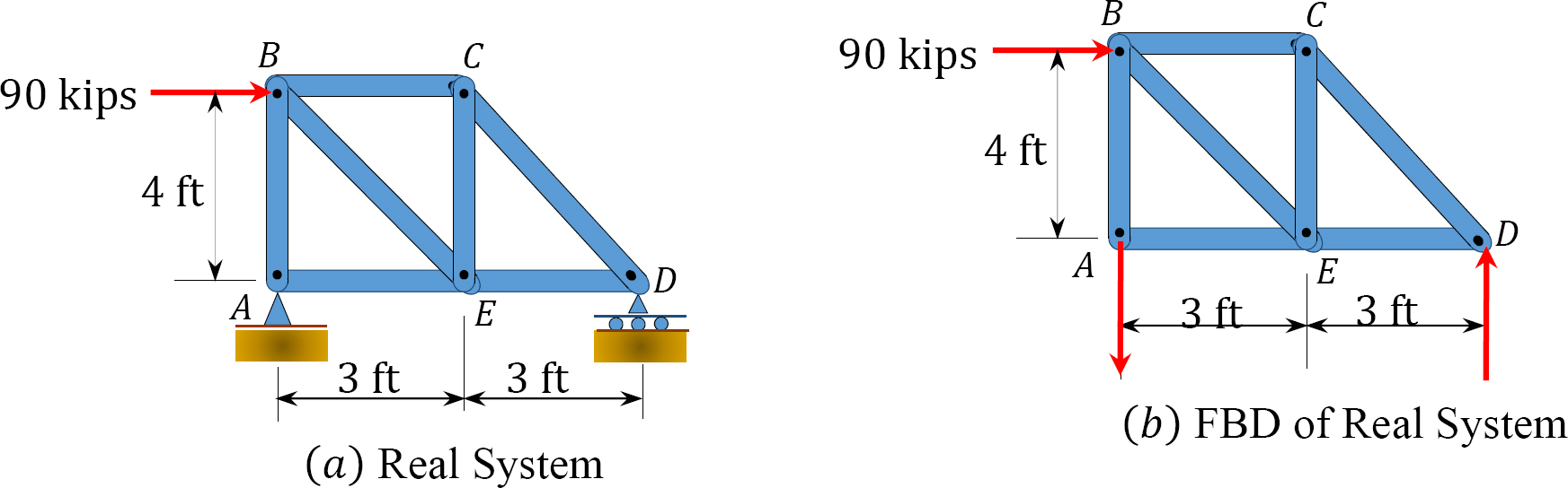
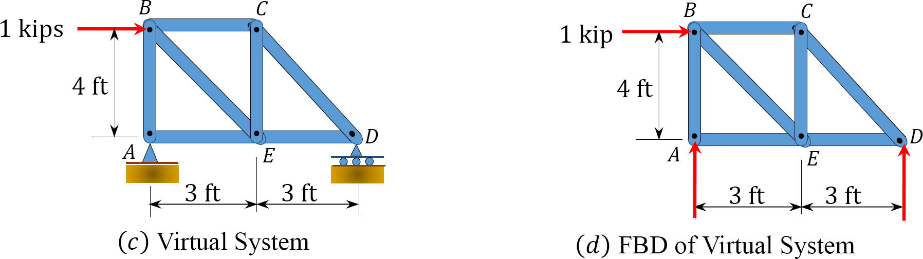
Using the virtual work method, determine the horizontal deflection at joint \(B\) of the truss shown in Figure 8.9a. \(E=12000 \mathrm{ksi} \text { and } A=3 \mathrm{in}^{2}\).

\(Fig. 8.9\). Truss.

Solution

Real and virtual systems. The real and virtual systems are shown in Figure 8.9. Notice that the real system consists of the external loading carried by the truss, as specified in the problem. The virtual system consists of a unit 1-k load applied at \(B\), where the deflection is desired, and a 1-k-ft moment applied also at \(B\), where the slope is required.

Truss analysis. The analysis of the real system used to obtain the forces in members is presented below. The forces in members in the virtual system are obtained by dividing the forces in the real system by the applied external load, as the deflection is desired for the same joint where the deflection is required.

Support reactions. The reactions are computed by the application of the equations of equilibrium, as follows:

\(\begin{array}{l}
+\curvearrowleft \sum M_{D}=0 \\
6 A_{y}-90(4)=0 \\
A_{y}=60 \text { kips } \quad \quad A_{y}=60 \text { kips } \downarrow \\
+\rightarrow \sum F_{x}=0 \\
-A_{x}+90=0 \\
A_{x}=90 \text { kips } \quad \quad A_{x}=90 \text { kips } \leftarrow \\
+\uparrow \sum F_{y}=0 \\
D_{y}-60=0 \\
D_{y}=60 \mathrm{kN} \quad \quad D_{y}=60 \text { kips } \uparrow
\end{array}\)

Joint \(A\).

\(\begin{array}{l}
+\uparrow \sum F_{y}=0 \\
F_{A B}-60=0 \\
F_{A B}=60 \mathrm{kips}
\end{array}\)

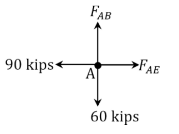
\(\begin{array}{l}
+\rightarrow \Sigma F_{x}=0 \\
F_{A E}-90=0 \\
F_{A E}=90 \mathrm{kips}
\end{array}\)

Joint \(B\).

\(\begin{array}{l}
+\uparrow \sum F_{y}=0 \\
-F_{B E} \sin 53.13^{\circ}-F_{B A}=0 \\
F_{B E}=-\frac{F_{B A}}{\sin 53.13^{\circ}}=-\frac{60}{\sin 53.13^{\circ}}=-75 \mathrm{kips}
\end{array}\)

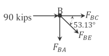
\(\begin{array}{l}
+\rightarrow \sum F_{x}=0 \\
F_{B E} \cos 53.13^{\circ}+90+F_{B C}=0 \\
F_{B C}=-F_{B E} \cos 53.13^{\circ}-90=-(-75) \cos 53.13^{\circ}-90=-45 \mathrm{kips}
\end{array}\)

Joint \(C\).

\(\begin{array}{l}
+\rightarrow \sum F_{x}=0 \\
F_{C D} \sin 36.87^{\circ}-F_{C B}=0 \\
F_{C D}=\frac{F_{C B}}{\sin 36.87^{\circ}}=-\frac{45}{\sin 36.87}=-75 \mathrm{kips}
\end{array}\)

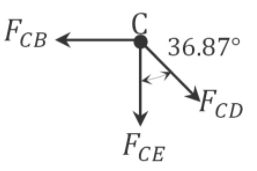
\(\begin{array}{l}
+\uparrow \sum F_{y}=0 \\
-F_{C E}-F_{C D} \cos 36.87^{\circ}=0 \\
F_{C E}=-F_{C D} \cos 36.87^{\circ}=-(-75) \cos 36.87^{\circ}=60 \mathrm{kips}
\end{array}\)

Joint \(D\).

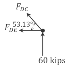
\(\begin{array}{l}
+\rightarrow \sum F_{x}=0 \\
-F_{D C} \cos 36.87^{\circ}-F_{D E}=0 \\
F_{D E}=-F_{D C} \cos 36.87^{\circ}=-(-75) \cos 36.87^{\circ}=60 \mathrm{kips}
\end{array}\)

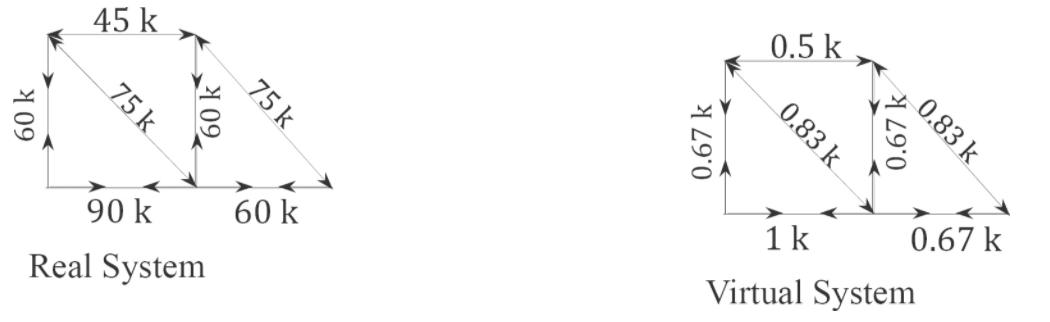
Horizontal deflection at \(B\). The desired horizontal deflection at joint \(B\) is computed using equation 8.17, as presented in Table 8.6.

\(Table 8.6\). Horizontal deflections.

Member	Length (ft)	N (kip)	N (kip)	NnL (k^2. ft)
AB	4	60	0.67	160.8
AE	3	90	1	270
BC	3	45	0.5	67.5
BE	5	75	0.83	311.25
CD	5	75	0.83	311.25
CE	4	60	0.67	160.8
DE	3	60	0.67	120.6
\(\sum{NnL}=1401.4\)

\(\begin{array}{l}
1\left(\Delta_{B}\right)=\frac{1}{E A} \sum \mathrm{NnL} \\
(1 \mathrm{k}) \Delta_{B}=\frac{1401.4}{12000\left(12^{2}\right)(3)\left(12^{-2}\right)} \\
\Delta_{B}=0.039 \mathrm{ft}=0.47 \mathrm{in} \quad \quad \Delta_{B}=0.47 \mathrm{in} \downarrow
\end{array}\)

Example 8.7

Using the virtual work method, determine the vertical deflection at joint \(D\) of the truss shown in Figure 8.10a. \(E=200 \mathrm{GPa} \text { and } A=5 \mathrm{~cm}^{2}\).

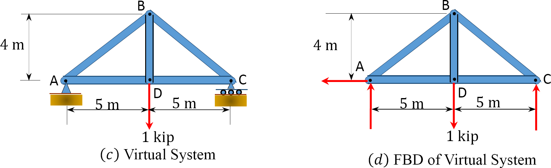
\(Fig. 8.10\). Truss.

Solution

Real and virtual systems. The real and virtual systems are shown in Figure 8.10. Notice that the real system consists of the external loading carried by the beam, as specified in the problem. The reactions in both supports in the real system are the same by reason of symmetry in loading and equal 60 kN. The virtual system consists of a unit 1-k load applied at \(B\), where the deflection is required, and a 1-k-ft moment applied at the same point, where the slope is to be determined. The bending moment at each portion of the beam with respect to the horizontal axis is presented in Table 8.7. Notice that the origin of the horizontal distance \(x\) for both the real and virtual system is at the free end, as shown in Figure 8.10.

Real system-truss analysis.

Joint \(A\).

\(\begin{array}{l}
+\uparrow \sum F_{y}=0 \\
F_{A B} \sin 38.66^{\circ}+60=0 \\
F_{A B}=-96.05 \mathrm{kN}
\end{array}\)

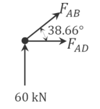
\(\begin{array}{l}
+\rightarrow \sum F_{x}=0 \\
F_{A B} \cos 38.66^{\circ}+F_{A D}=0 \\
F_{A D}=-F_{A B} \cos 38.66^{\circ} \\
\quad=-(-96.05) \cos 38.66^{\circ}=75 \mathrm{kN}
\end{array}\)

Joint \(D\).

\(\begin{array}{l}
+\uparrow \sum F_{y}=0 \\
F_{D B}=0 \\
+\rightarrow \sum F_{x}=0 \\
-F_{D A}+F_{D C}=0 \\
F_{D C}=F_{D A}=75 \mathrm{kN}
\end{array}\)

Virtual system truss analysis.

Joint \(A\).

\(\begin{array}{l}
+\uparrow \sum F_{y}=0 \\
F_{A B} \sin 38.66^{\circ}+0.5=0 \\
F_{A B}=-0.08 \mathrm{kN}
\end{array}\)

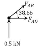
\(\begin{array}{l}
+\rightarrow \sum F_{x}=0 \\
F_{A B} \cos 38.66^{\circ}+F_{A D}=0 \\
F_{A D}=-F_{A B} \cos 38.66^{\circ} \\
\quad=-(-0.08) \cos 38.66^{\circ}=0.062 \mathrm{kN}
\end{array}\)

Joint \(D\).

\(\begin{array}{l}
+\uparrow \sum F_{y}=0 \\
F_{D B}-1=0 \\
F_{D B}=1 \mathrm{kN}
\end{array}\)

\(\begin{array}{l}
+\rightarrow \sum F_{x}=0 \\
-F_{D A}+F_{D C}=0 \\
F_{D C}=F_{D A}=0.062 \mathrm{kN}
\end{array}\)

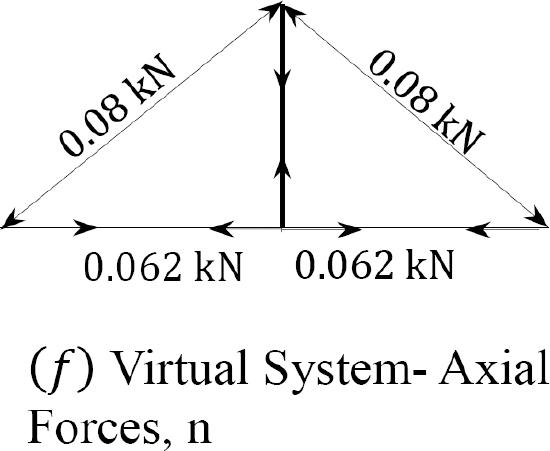
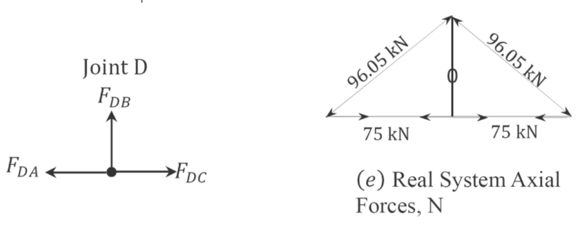
Vertical deflection at \(D\). The desired vertical deflection at joint \(D\) is calculated using equation 8.17, as presented in Table 8.7.

\(Table 8.7\). Vertical deflections.

Member	Length (m)	N	n	NnL (kN^2.m)
AB	6.4	-96.05	-0.08	49.18
AD	5	75	0.062	23.25
BC	6.4	-96.05	-0.08	49.18
BD	4	0	1	0
DC	5	75	0.062	23.25
\(\sum{NnL}=144.86\)

\(\begin{array}{l}
1\left(\Delta_{D}\right)=\frac{1}{E A} \sum N n L \\
(1 k N) \Delta_{D}=\frac{144.86}{200\left(10^{6}\right)(0.0005)} k N . m \\
\Delta_{D}=1.45 \times 10^{-3} m=1.45 \mathrm{~mm} \quad \quad \Delta_{D}=1.45 \mathrm{~mm} \downarrow
\end{array}\)