8.2: Energy Methods

The energy method for the determination of deflection is based on Alberto Castigliano’s second theorem, which was published in 1879. The theorem states the following:

The deflection or rotation in a specified direction and at a specified point in a linear elastic, statically determinate structure subjected to a given force or couple is equal to the partial derivative of the total external work or the total internal energy, with respect to the applied force or couple in the direction of the force or couple.

Castigliano’s second theorem, with respect to the applied force, can be expressed mathematically, as follows:

\[\Delta=\frac{\partial W}{\partial P}=\frac{\partial U}{\partial P}\]

where

• \(\Delta\) = deflection at the point of application of the load \(P\) in the direction of the load \(P\).
• \(W\) = work done.
• \(U\) = strain energy.

Energy Method Formulation for Beams and Frames

Equation 8.18 can be mathematically manipulated to include moment and is written as follows:

\[\Delta=\frac{\partial U}{\partial P}=\frac{\partial U}{\partial M} \times \frac{\partial M}{\partial P}\]

The total internal work done or strain energy stored in a beam or frame due to gradually applied real loads can be expressed as follows:

\[W=U=\int \frac{M^{2}}{2 E I} d x\]

The partial derivative of equation 8.20, with respect to the moment, is as follows:

\[\frac{\partial U}{\partial M}=\int\left(\frac{2 M}{2 E I}\right) d x=\int\left(\frac{M}{E I}\right) d x\]

Substituting equation 8.21 into equation 8.19 yields the following equation for the computation of deflection for beams and frames by the energy method:

\[\Delta=\int\left(\frac{M}{E I}\right)\left(\frac{\partial M}{\partial P}\right) d x\]

With respect to the applied couple, Castigliano’s second theorem can be expressed mathematically as follows:

\[\theta=\frac{\partial W}{\partial M^{\prime}}=\frac{\partial U}{\partial M^{\prime}}\]

where \(\theta\) = rotation at the point of application and direction of the couple \(M^{\prime}\).

Equation 8.23 can be mathematically manipulated to include the moment, as follows:

\[\theta=\frac{\partial U}{\partial M^{\prime}}=\frac{\partial U}{\partial M} \times \frac{\partial M}{\partial M^{\prime}}\]

Substituting equation 8.21 into equation 8.24 suggests the following equation for the computation of slopes for beams and frames by the energy method:

\[\theta=\int\left(\frac{M}{E I}\right)\left(\frac{\partial M}{\partial M^{\prime}}\right) d x\]

Example 8.8

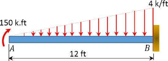
Using Castigliano’s second theorem, determine the deflection and the slope at the free end of the cantilever beam shown in Figure 8.11a.

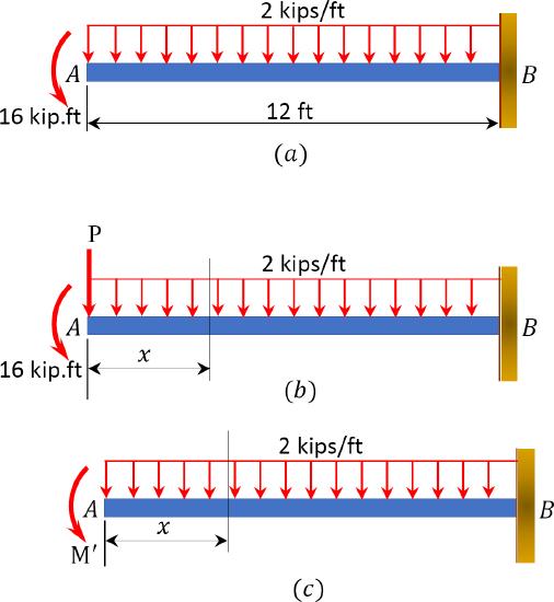
\(Fig. 8.11\). Cantilever beam.

Solution

Placement of imaginary force \(P\) and couple \(M^{\prime}\). The force \(P\) and the moment \(M^{\prime}\) are placed at point \(A\), where the deflection and slope are desired, as shown in Figure 8.11b and Figure 8.11c, respectively.

Bending moment. To determine the deflection, write the bending moment equation for the beam as a function of the force \(P\). To determine the slope, write the bending moment equation for the beam as a function of \(M^{\prime}\). The \(x\) coordinates for the moment equations are also shown in Figure 8.11b and Figure 8.11c. Compute the partial derivatives \(\frac{\partial M}{\partial P}\) and \(\frac{\partial M}{\partial M^{\prime}}\), and then apply Castigliano’s equation 8.22 and equation 8.25 to determine the deflection and slope.

Deflection at \(A\).

\(\begin{array}{l}
M=-16-P x-x^{2} \\
\frac{\partial M}{\partial P}=-x
\end{array}\)

Setting \(P = 0\) and applying Castigliano’s theorem suggests the following:

\(\begin{aligned}
\Delta_{A} &=\int_{0}^{L}\left(\frac{M}{E I}\right)\left(\frac{\partial M}{\partial P}\right) d x \\
\Delta_{A} &=\int_{0}^{12}\left(\frac{-16-x^{2}}{E I}\right)(-x) d x \\
&=\frac{6336 \mathrm{k} \cdot \mathrm{ft}^{3}}{E I}=\frac{6336(12)^{3} \mathrm{k} \cdot \mathrm{ft}^{3}}{(29000)(1500)}=0.252 \mathrm{in} \quad \Delta_{A}=0.252 \mathrm{in} \downarrow
\end{aligned}\)

Slope at \(A\).

\(\begin{array}{l}
M=-M^{\prime}-x^{2} \\
\frac{\partial M}{\partial M^{\prime}}=-1
\end{array}\)

Setting \(M^{\prime} = 16\) k. ft and applying Castigliano’s theorem suggests the following:

\(\begin{array}{l}
\qquad \theta_{A}=\int_{0}^{L}\left(\frac{M}{E I}\right)\left(\frac{\partial M}{\partial M^{\prime}}\right) d x \\
\theta_{A}=s \int_{0}^{12}\left(\frac{-16-x^{2}}{E I}\right)(-1) d x \\
=\frac{768 \mathrm{k} \cdot \mathrm{ft}^{2}}{E I}=\frac{768(12)^{2}}{(29000)(1500)}=0.0025 \mathrm{rad}
\end{array}\)

Example 8.9

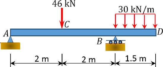
Using Castigliano’s second theorem, determine the deflection at point \(A\) of the beam with the overhang shown in Figure 8.12a.

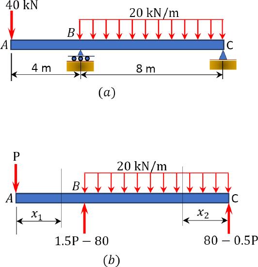
\(Fig. 8.12\). Beam with overhang.

Solution

Placement of imaginary force \(P\). The force \(P\) is placed at point \(A\), where the deflection is desired, as shown in Figure 8.12b. The \(x\) coordinates for the moment equations are also shown in this figure.

Bending moment. Compute the support reactions and write the bending moment equations for segments \(AB\) and \(BC\) of the beam as a function of the force \(P\). The \(x\) coordinates for the moment equations are also shown in Figure 8.12b. Compute the partial derivatives \(\frac{\partial M}{\partial P^{\prime}}\) and then apply Castigliano’s equation 8.22 to compute the deflection.

Segment \(AB\). \((0 < x_{1} < 4)\)

\(\begin{array}{l}
M_{1}=-P x_{1} \\
\frac{\partial M_{1}}{\partial P}=-x_{1}
\end{array}\)

Segment \(BC\). \((0 < x_{2} < 8)\)

\(\begin{array}{l}
M_{2}=(80-0.5 P) x_{2}-10 x_{2}^{2} \\
\frac{\partial M_{2}}{\partial P}=-0.5 x_{2}
\end{array}\)

Setting \(P = 40\) kN and applying Castigliano’s theorem suggests the following:

\(\begin{aligned}
\Delta_{A} &=\int_{0}^{L}\left(\frac{M}{E I}\right)\left(\frac{\partial M}{\partial P}\right) d x \\
\Delta_{A} &=\int_{0}^{4}\left(\frac{-40 x_{1}}{E I}\right)\left(-x_{1}\right) d x+\int_{0}^{8}\left(\frac{100 x_{2}-10 x_{2}^{2}}{E I}\right)\left(-0.5 x_{2}\right) d x \\
&=\frac{-2560 \mathrm{kN} \cdot \mathrm{m}^{3}}{E I}=\frac{-2560 \mathrm{kN} \cdot \mathrm{m}^{3}}{\left(200 \times 10^{6} \mathrm{kN} / \mathrm{m}^{2}\right)\left(800 \times 10^{6} \mathrm{~mm}^{4}\right)\left(10^{-12} \mathrm{~m}^{4} / \mathrm{mm}^{4}\right)}=-0.016 \mathrm{~m} \\
& \Delta_{A}=16 \mathrm{~mm} \uparrow
\end{aligned}\)

Example 8.10

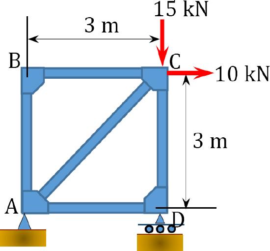
Using Castigliano’s second theorem, determine the rotation of joint \(C\) of the frame shown in Figure 8.13a.

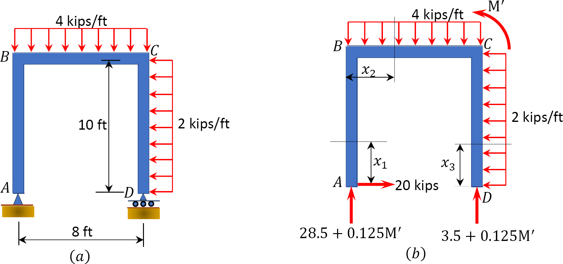
\(Fig. 8.13\). Frame.

Solution

Placement of imaginary couple \(M^{\prime}\). The couple force \(M^{\prime}\) is placed at point \(C\), where the rotation is desired, as shown in Figure 8.13b.

Bending moment. Compute the support reactions and write the bending moment equations for the columns \(AB\) and \(DC\) and the beam \(BC\) of the frame as a function of the couple \(M^{\prime}\). Compute the partial derivatives \(\frac{\partial M}{\partial M^{\prime}}\) and then apply Castigliano’s equation 8.25 for the computation of rotation.

Column \(AB\). \((0 < x_{1} < 10)\)

\(\begin{array}{l}
M_{1}=-20 x_{1} \\
\frac{\partial M_{1}}{\partial M^{\prime}}=0
\end{array}\)

Beam \(BC\). \((0 < x_{2} < 8)\)

\(\begin{array}{l}
M_{2}=\left(28.5+0.125 \mathrm{M}^{\prime}\right) x_{2}-2 x_{2}^{2} \\
\frac{\partial M_{2}}{\partial M^{\prime}}=0.125 x_{2}
\end{array}\)

Column \(DC\). \((0 < x_{3} < 10)\)

\(\begin{array}{l}
M_{3}=-x_{3}^{2} \\
\frac{\partial M_{3}}{\partial M^{\prime}}=0
\end{array}\)

Setting \(M^{\prime} = 16\) k. ft and applying Castigliano’s theorem suggests the following:

\(\begin{aligned}
\theta_{A} &=\int_{0}^{L}\left(\frac{M}{E I}\right)\left(\frac{\partial M}{\partial M^{\prime}}\right) d x \\
\theta_{A} &=\int_{0}^{10}\left(\frac{-20 x_{1}}{E I}\right)(0) d x+\int_{0}^{8}\left(\frac{28.5 x_{2}-2 x_{2}^{2}}{E I}\right)\left(0.125 x_{2}\right) d x+\int_{0}^{10}\left(\frac{-x_{3}^{2}}{E I}\right)(0) d x \\
&=\frac{351.57 \mathrm{k} . \mathrm{ft}^{2}}{E I}=\frac{351.57(12)^{2}}{(29000)(100)}=0.017 \mathrm{rad}
\end{aligned}\)

Energy Method Formulation for Trusses

Equation 8.18 can be mathematically manipulated to include axial force, as follows:

\[\Delta=\frac{\partial U}{\partial P}=\frac{\partial U}{\partial N} \times \frac{\partial N}{\partial P}\]

The total internal work done or strain energy stored in members of a truss due to gradually applied external loads is as follows:

\[W=U=\sum \frac{N^{2} L}{2 A E}\]

The partial derivative of equation 8.27, with respect to the axial load, is as follows:

\[\begin{array}{l}
\frac{\partial U}{\partial N}=\sum \frac{2 N L}{2 A E}=\sum \frac{N L}{A E}
\end{array}\]

To determine the deflection at any joint of a truss, use the energy method by substituting equation 8.28 into equation 8.26 to obtain the following equation:

\[\Delta=\sum\left(\frac{N L}{A E}\right)\left(\frac{\partial N}{\partial P}\right)\]

where

\(N\) = internal axial force in each member due to external load.

\(\frac{\partial N}{\partial P}\) = axial force in each member due to unit load applied at the joint and in the direction of the required deflection.

\(L\) = length of member.

\(A\) = area of a member.

\(E\) = modulus of elasticity of a member.

Example 8.11

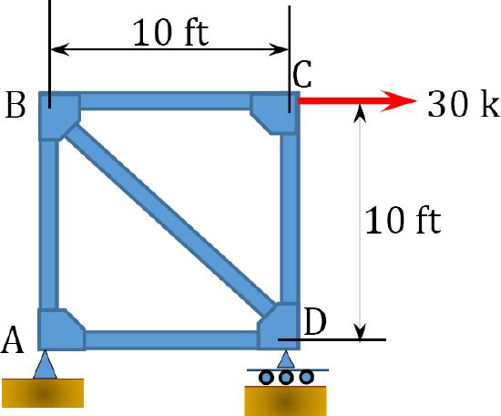
Using Castigliano’s second theorem, determine the horizontal deflection at joint \(C\) of the truss shown in Figure 8.14a.

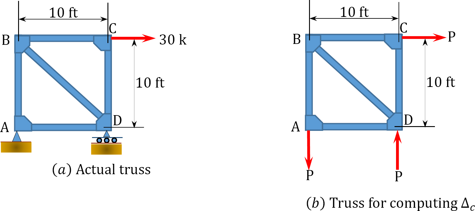
\(Fig. 8.14\). Truss.

Solution

Placement of imaginary force \(P\). The force \(P\) is placed as a replacement for the 30k force at point \(C\), where the horizontal deflection is desired, as shown in Figure 8.14b.

Member axial forces. Compute the support reactions and obtain the member-axial forces in terms of the imaginary force \(P\). Member-axial forces are determined by using the method of joint, as shown below. To find the horizontal deflection at \(C\), compute the partial derivatives \(\frac{\partial M}{\partial P}\) and apply Castigliano’s equation 8.22. Member lengths, axial forces, and partial derivatives with respect to the fictitious force \(P\) are shown in Table 8.8.

Analysis of truss (fig. 8.14b).

Joint \(A\).

\(\begin{array}{l}
+\uparrow \sum F_{y}=0 \\
N_{A B}-P=0 \\
N_{A B}=P
\end{array}\)

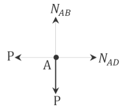
\(\begin{array}{l}
+\rightarrow \sum F_{x}=0 \\
N_{A D}-P=0 \\
N_{A D}=P
\end{array}\)

Joint \(B\).

\(\begin{array}{l}
+\uparrow \sum F_{y}=0 \\
-N_{B A}-N_{B D} \cos 45^{\circ}=0 \\
N_{B D}=-\frac{N_{B A}}{\cos 45^{\circ}}=-\frac{P}{\cos 45^{\circ}}=-1.41 P
\end{array}\)

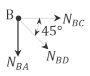
\(\begin{array}{l}
+\rightarrow \sum F_{x}=0 \\
N_{B C}+N_{B D} \cos 45^{\circ}=0 \\
N_{B C}=-N_{B D} \cos 45^{\circ}=-(-1.41 P) \cos 45^{\circ}=P
\end{array}\)

Joint \(C\).

\(+\uparrow \sum F_{y}=0\)

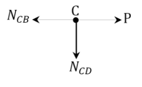
\(\begin{array}{l}
N_{C D}=0 \\
+\rightarrow \sum F_{x}=0 \\
-N_{C B}+P=0 \\
N_{C B}=P
\end{array}\)

\(Table 8.8\). Member lengths, axial forces, and partial derivatives with respect to the fictitious force P.

Member	L (ft) (ft)	N (kip) (kip)	\[\frac{\partial N}{\partial P}\nonumber\] (kip/kip)	N (P=30k) (kip)	\[N (\partial N/ \partial P) L\nonumber\] (kip. ft)
AB	10	P	1	30	300
AD	10	P	1	30	300
BC	10	P	1	30	300
BD	14.14	-1.14P	-1.14	-34.2	551.29
CD	10	0	0	0	0
\(\sum{N(\frac{\partial N}{\partial P})L}=1451.29\)

\(\Delta_{c}=\frac{1}{E A} \sum N\left(\frac{\partial N}{\partial P}\right) L=\frac{1451.29}{E A} \mathrm{k} . \mathrm{ft}=\frac{1451.29(12)}{(29,000)(0.6)}=0.083 \mathrm{ft}=1 \mathrm{in} \quad \Delta_{c}=1 \mathrm{in} \rightarrow\)

Example 8.12

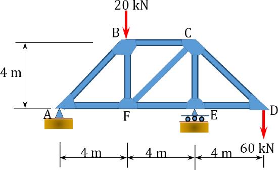
Using Castigliano’s second theorem, determine the vertical deflection at joint \(F\) of the truss shown in Figure 8.15a.. Members have the same cross-sectional area of 600 mm² and \(E\) = 200 GPa.

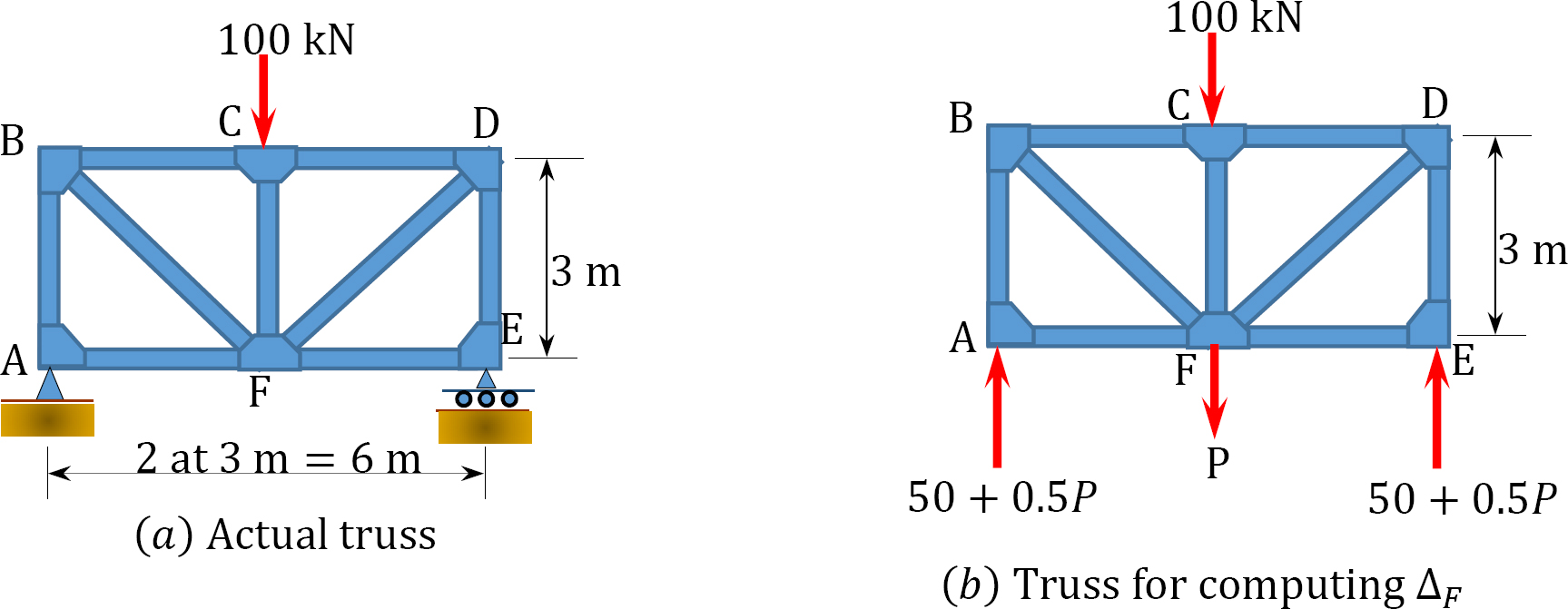
\(Fig. 8.15\). Truss.

Solution

Placement of imaginary force \(P\). The force \(P\) is placed at joint \(F\), where the vertical deflection is desired, as shown in Figure 8.15b.

Member axial forces. Compute support reactions and obtain member-axial forces in terms of the imaginary force \(P\). Member-axial forces are determined by using the method of joint, as shown below. To find the vertical deflection at \(F\), compute the partial derivatives \(\frac{\partial M}{\partial P}\) and apply Castigliano’s equation 8.22. Member lengths, axial forces, and partial derivatives with respect to the fictitious force \(P\) are shown in Table 8.9.

Analysis of truss (fig. 8.15b).

Joint \(A\).

\(\begin{array}{l}
+\uparrow \sum F_{y}=0 \\
N_{A B}+50+0.5 P=0 \\
N_{A B}=-50-0.5 P
\end{array}\)

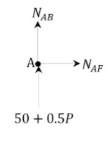
\(+\rightarrow \sum_{N_{A F}} F_{x}=0\)

Joint \(B\).

\(\begin{array}{l}
+\uparrow \sum F_{y}=0 \\
-N_{B A}-N_{B F} \cos 45^{\circ}=0 \\
N_{B F}=-\frac{N_{B A}}{\cos 45^{\circ}}=-\frac{(-50-0.5 P)}{\cos 45^{\circ}}=70.71+0.7071 P
\end{array}\)

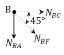
\(\begin{array}{l}
+\rightarrow \sum F_{x}=0 \\
N_{B C}+N_{B F} \cos 45^{\circ}=0 \\
N_{B C}=-N_{B F} \cos 45^{\circ}=-(70.71+0.7071 P)
\end{array}\)

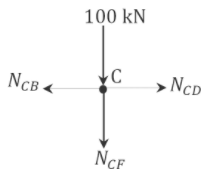
Joint \(C\).

\(\begin{array}{l}
+\uparrow \sum F_{y}=0 \\
-N_{C F}-100=0 \\
N_{C F}=-100 \mathrm{kN}
\end{array}\)

\(\begin{array}{l}
+\rightarrow \sum F_{x}=0 \\
-N_{C B}+N_{C D}=0 \\
N_{C D}=N_{C B}=-(70.71+0.7071 P)
\end{array}\)

\(Table 8.9\). Member lengths, axial forces, and partial derivatives with respect to the fictitious force \(P\).

Member	L (m)	N (kN)	\[\frac{\partial N}{\partial P}\nonumber\] (kN/kN)	N(P=0) (kN)	\[N(\partial N/\partial P)L\nonumber\] (kN.m)
AB	3	-50-0.5P	-0.5	-50	75
AF	3	0	0	0	0
BC	3	-70.71-0.7071P	-0.7071	-70.71	150
BF	4.24	70.71+0.7071P	0.7071	70.71	212
CF	3	100	0	100	0
CD	3	-70.71-0.7071P	-0.7071	-70.71	150
DF	4.24	70.71+0.7071P	0.7071	70.71	212
DE	3	-50-0.5P	-0.5	-50	75
EF	3	0	0	0	0
\(\sum{N(\frac{\partial N}{\partial P})L}=874\)

\(\Delta_{c}=\frac{1}{E A} \sum N\left(\frac{\partial N}{\partial P}\right) L=\frac{874}{E A} \mathrm{kN} \cdot \mathrm{m}=\frac{1451.29(12)}{(29,000)(0.6)}=0.083 \mathrm{ft}=1 \text { in } \quad \Delta_{c}=1 \text { in } \rightarrow\)

Chapter Summary

Principle of virtual work: The principle of virtual work states that if a body acted upon by several external forces is in a state of equilibrium and is subjected to a small virtual displacement, the virtual work done by the externally applied forces is zero. This principle can be expressed mathematically, as follows:

\(W_{e}=W_{i}\)

The expressions for the determination of deflection by virtual work method for beams and trusses are as follows:

\(\begin{array}{l}
\text {Beams and Frames:} \quad \quad 1(\Delta)=\int_{0}^{L} \frac{M m_{v}}{E T} d x \\
\quad \text {Trusses:} \quad 1(\Delta)=\sum n_{i}\left(\frac{N_{i} L_{i}}{A_{i} E_{i}}\right)
\end{array}\)

Principle of conservation of energy: The principle of conservation of energy states that the work done by external forces acting on an elastic body in equilibrium are equal to the strain energy stored in the body. This principle can be expressed mathematically, as follows:

\(W\left(\text { or } U_{e}\right)=U_{i}\)

The energy method for the determination of deflection is based on Alberto Castigliano’s second theorem. The theorem states that the deflection in a specified direction and at a specified point in a linear elastic structure subjected to a given force is equal to the partial derivative of the total external work or the total internal energy with respect to the applied force. The expressions for the determination of deflection by Castigliano’s second theorem for beams and trusses are as follows:

\(\begin{array}{l}
\text {Beams and Frames:} \quad \quad \Delta=\int\left(\frac{M}{E I}\right)\left(\frac{\partial M}{\partial P}\right) d x \\
\quad \text {Trusses:} \quad \Delta=\sum\left(\frac{N L}{A E}\right)\left(\frac{\partial N}{\partial P}\right)
\end{array}\)

Practice Problems

8.1 Using the virtual work method, determine the slope and deflection at point \(A\) of the cantilever beams shown in Figure P8.1 and Figure P8.2.

\(Fig. P8.1\). Cantilever beam.

\(Fig. P8.2\). Cantilever beam.

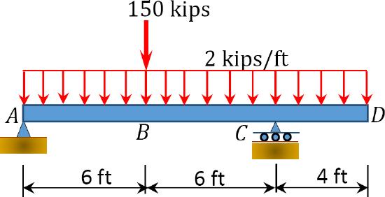
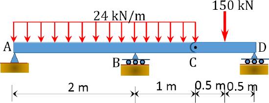
8.2 Determine the deflection at point D of the beams shown in Figure P8.3 and Figure P8.4.

\(Fig. P8.3\). Beam.

\(Fig. P8.4\). Beam.

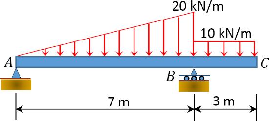
8.3 Using the energy method, determine the slope at support \(B\) of the beams shown in Figure P8.5 and Figure P8.6.

\(Fig. P8.5\). Beam.

\(Fig. P8.6\). Beam.

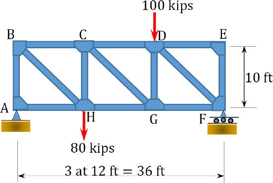
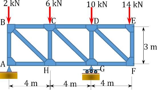
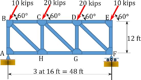
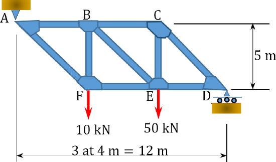
8.4 Using the virtual work method, determine the deflection at point \(H\) of the trusses shown in Figure P8.7 through Figure P8.10.

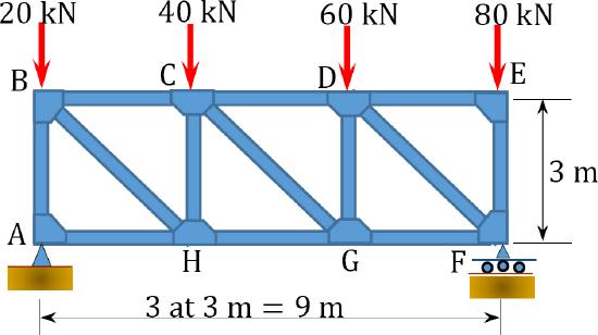
\(Fig. P8.7\). Truss.

\(Fig. P8.8\). Truss.

\(Fig. P8.9\). Truss.

\(Fig. P8.10\). Truss.

8.5 Using the energy method, determine the deflection at point \(F\) of the trusses shown in Figure P8.11 and Figure P8.12.

\(Fig. P8.11\). Truss.

\(Fig. P8.12\). Truss.

8.6 Using the virtual work method, determine the horizontal deflection at joint \(C\) of the trusses shown in Figure P8.13 and Figure P8.14.

\(Fig. P8.13\). Truss.

\(Fig. P8.14\). Truss.