9.4: Uses of Influence Lines

Uses of Influence Lines to Determine Response Functions of Structures Subjected to Concentrated Loads

The magnitude of a response function of a structure due to concentrated loads can be determined as the summation of the product of the respective loads and the corresponding ordinates of the influence line for that response function. Example 9.5 and example 9.6 illustrate such cases.

Example 9.8

A simple beam is subjected to three concentrated loads, as shown in Figure 9.15a. Determine the magnitudes of the reactions and the shear force and bending moment at the midpoint of the beam using influence lines.

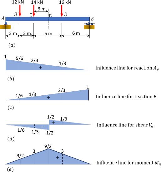
\(Fig. 9.15\). Simple beam.

Solution

First, draw the influence line for the support reactions and for the shearing force and the bending moment at the midpoint of the beam (see Fig. 9.15b, Fig. 9.15c, Fig. 9.15d, and Fig. 9.15e). Once the influence lines for the functions are drawn, compute the magnitude of the response functions, as follows:

Magnitude of the support reactions using the influence line diagrams in Figure 9.15b and Figure 9.15c.

\(\begin{array}{l}
A_{y}=(12)\left(\frac{5}{6}\right)+(14)\left(\frac{2}{3}\right)+(16)\left(\frac{1}{3}\right)=24.67 \mathrm{kN} \\
E_{y}=(12)\left(\frac{1}{6}\right)+(14)\left(\frac{1}{3}\right)+(16)\left(\frac{2}{3}\right)=17.33 \mathrm{kN}
\end{array}\)

Magnitude of the shear force at section n using the influence line diagram in Figure 9.15d.

\(V_{n}=(12)\left(-\frac{1}{6}\right)+(14)\left(-\frac{1}{3}\right)+(16)\left(\frac{1}{3}\right)=-1.33 \mathrm{kN}\)

Magnitude of the bending moment at section \(n\) using the influence line diagram of Figure 9.15e.

\(M_{n}=(12)\left(\frac{3}{2}\right)+(14)(3)+(16)(3)=108 \mathrm{kN} \cdot \mathrm{m}\)

Example 9.9

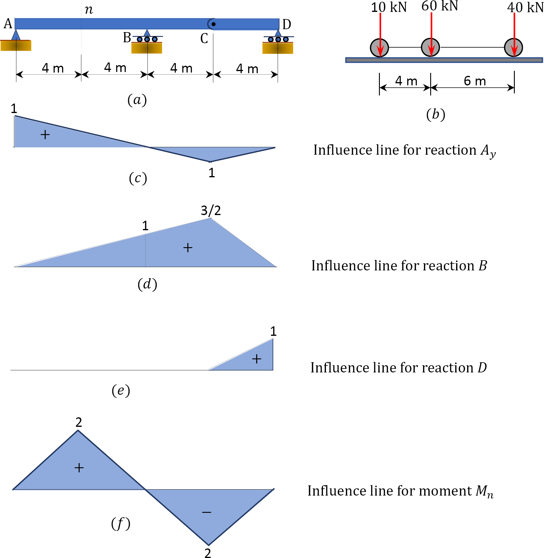
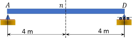
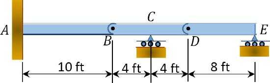
A compound beam is subjected to three concentrated loads, as shown in Figure 9.16a. Using influence lines, determine the magnitudes of the shear and the moment at \(A\) and the support reaction at \(D\).

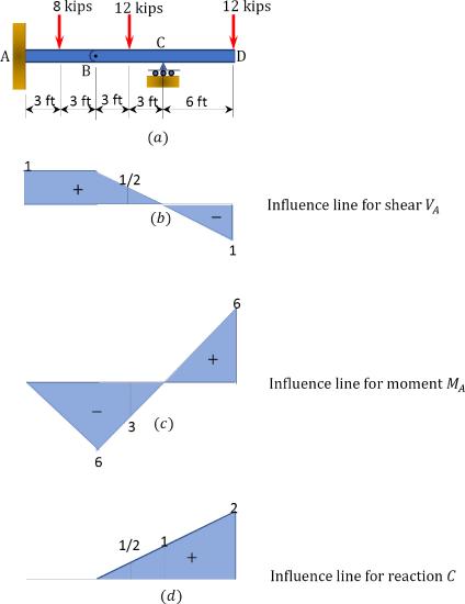
\(Fig. 9.16\). Compound beam.

Solution

First, draw the influence line for the shear force \(V_{A}\), bending moment \(M_{A}\), and reaction \(C_{y}\). The influence lines for these functions are shown in Figure 9.16b, Figure 9.16c, and Figure 9.16d. Then, compute the magnitude of these response functions, as follows:

The magnitude of the shear at section \(n\) using the influence line diagram in Figure 9.16b.

\(V_{A}=(8)(1)+(12)\left(\frac{1}{2}\right)+-(12)(1)=26 \text { kips }\)

The magnitude of the bending moment at section n using the influence line diagram in Figure 9.16c.

 

Magnitude of the support reaction \(C_{y}\) using the influence line diagram in Figure 9.16d.

\(C_{y}=(12)\left(\frac{1}{2}\right)+(12)(2)=30 \mathrm{kips}\)

Uses of Influence Lines to Determine Response Functions of Structures Subjected to Distributed Loads

The magnitude of a response function of a structure subjected to distributed loads can be determined as the product of the intensity of the distributed load and the area of the influence line. Consider a beam subjected to a uniform load \(\omega_{x}\), as shown in Figure 9.17a. First, convert the uniform load to an equivalent concentrated load. The equivalent elementary concentrated load for a distributed load acting on a differential length \(dx\) is as follows:

\[d P=\omega_{x} d x\]

The magnitude of the response function (\(rf\)) due to the elementary concentrated load acting on the structure can be expressed as follows:

\[r f=\left(\omega_{x} d x\right)(y)\]

where

\(y\) = the ordinate of the influence line at the point of application of the load \(dP\).

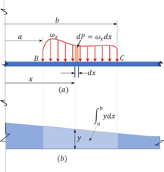
\(Fig. 9.17\). Beam subjected to uniform load.

The total response function (\(RF\)) due to the distributed load acting at the segment \(BC\) of the beam is obtained by integration, as follows:

\[R F=\int_{B}^{C}\left(\omega_{x}\right)(y) d x=\omega_{x} \int_{B}^{C}(y) d x\]

The integral \(\int_{B}^{C}(y) d x\) is the area under the portion of the influence line corresponding to the loaded segment of the beam (see the shaded area in Fig. 9.17b).

Example 9.10

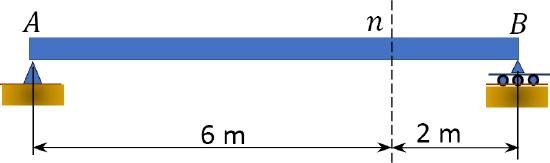
Using influence lines, determine the shear force and the bending moment at the midpoint of the loaded simple beam, as shown in Figure 9.18a.

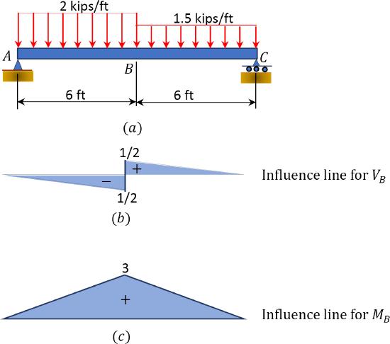
\(Fig. 9.18\). Loaded simple beam.

Solution

First, draw the influence line for the shear force and bending moment at the midspan of the beam. The influence lines for these functions are shown in Figure 9.18b and Figure 9.18c. Then, compute the magnitude of these response functions, as follows:

From the influence line diagram, as shown in Figure 9.18b, the magnitude of the shear at \(B\) is as follows:

\(V_{B}=(2)\left(-\frac{1}{2} \times 6 \times \frac{1}{2}\right)+(1.5)\left(\frac{1}{2} \times 6 \times \frac{1}{2}\right)=-0.75 \mathrm{kip}\)

The magnitude of the bending moment at point \(B\), using influence line diagram in Figure 9.18c, is as follows:

\(M_{B}=(2)\left(\frac{1}{2} \times 6 \times 3\right)+(1.5)\left(\frac{1}{2} \times 6 \times 3\right)=31.5 \text { kip. } \mathrm{ft}\)

Example 9.11

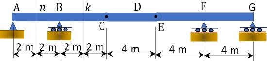
A compound beam is subjected to a combined loading, as shown in Figure 9.19a. Using influence lines, determine the magnitudes of the reactions at supports \(A\), \(B\), and \(C\).

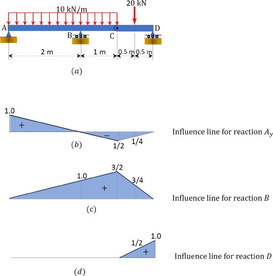
\(Fig. 9.19\). Compound beam subjected to combined loading.

Solution

The magnitude of the support reaction \(A_{y}\), using the influence line diagram in Figure 9.19b.

\(A_{y}=(10)\left(\frac{1}{2}\right)(2)(1)+(10)\left(\frac{1}{2}\right)(1)\left(-\frac{1}{2}\right)+(20)\left(-\frac{1}{4}\right)=2.5 \mathrm{kN}\)

The magnitude of the support reaction \(B_{y}\), using the influence line diagram in Figure 9.19c.

\(B_{y}=(10)\left(\frac{1}{2}\right)(3)\left(\frac{3}{2}\right)+(20)\left(\frac{3}{4}\right)=37.5 \mathrm{kN}\)

The magnitude of the support reaction \(D_{y}\), using the influence line diagram of Figure 9.19d.

\(D_{y}=(20)\left(\frac{1}{2}\right)=10 \mathrm{kN}\)

Use of Influence Lines to Determine the Maximum Effect at a Point Due to Moving Concentrated Loads

In the analysis and design of structures, such as bridges and cranes subjected to moving loads, it is often desirable to find the position of the moving load(s) that will produce a maximum influence at a point. For some structures, this can be determined by mere inspection, while for most others it may require a trial-and-error process using influence lines. Examples 9.12 and 9.13 illustrate the trial-and-error process involved when using influence lines to compute the magnitude of certain functions of a beam subjected to a series of concentrated moving loads.

Example 9.12

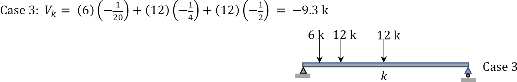
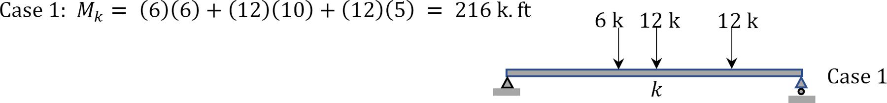
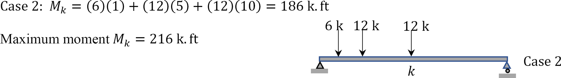
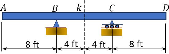
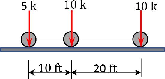
Using influence lines, determine the shear force and bending moment at the midpoint \(k\) of a beam shown in Figure 9.20a. The beam is subjected to a series of moving concentrated loads, which are shown in Figure 9.20b.

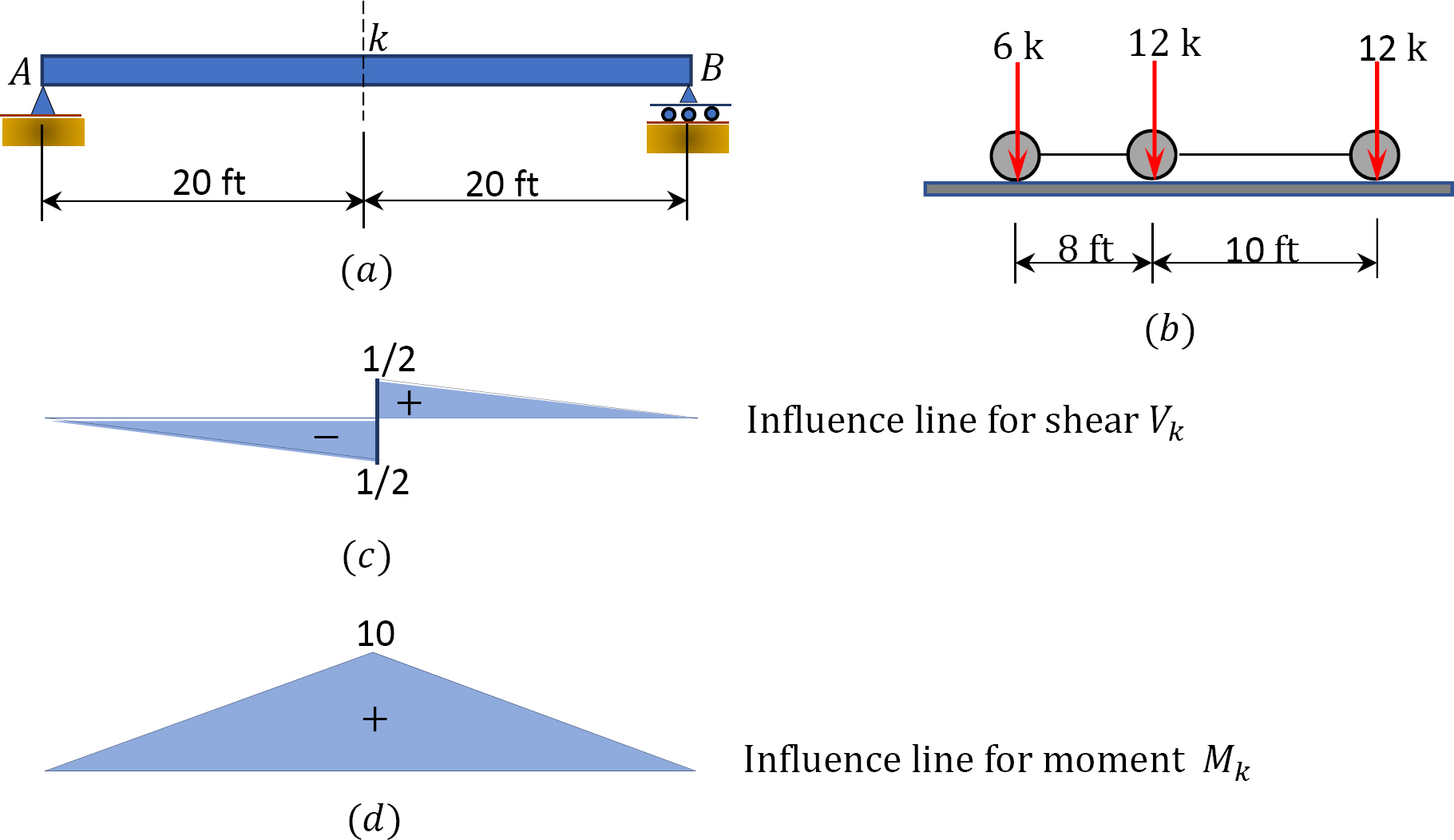
\(Fig. 9.20\). Beam.

Solution

Maximum shear \(V_{k}\) from Figure 9.20c.

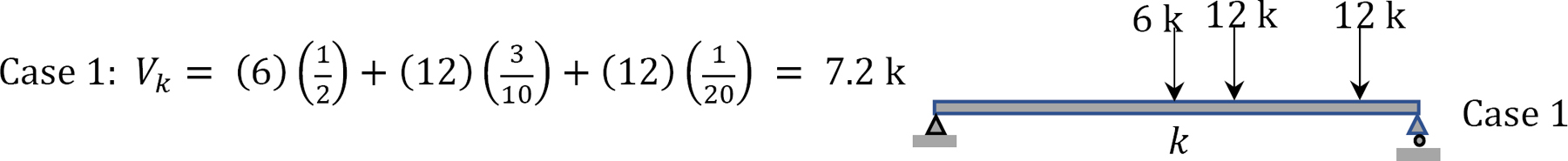
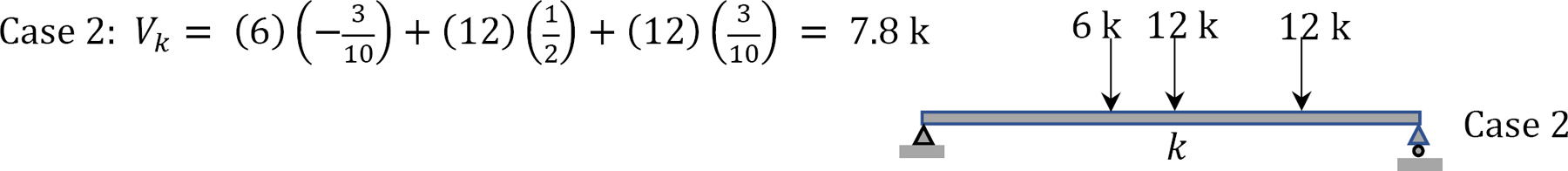
Maximum positive shear = 7.8 k

Maximum negative shear = 9.3 k

Maximum moment \(M_{k}\) from Figure 9.20d.

Example 9.13

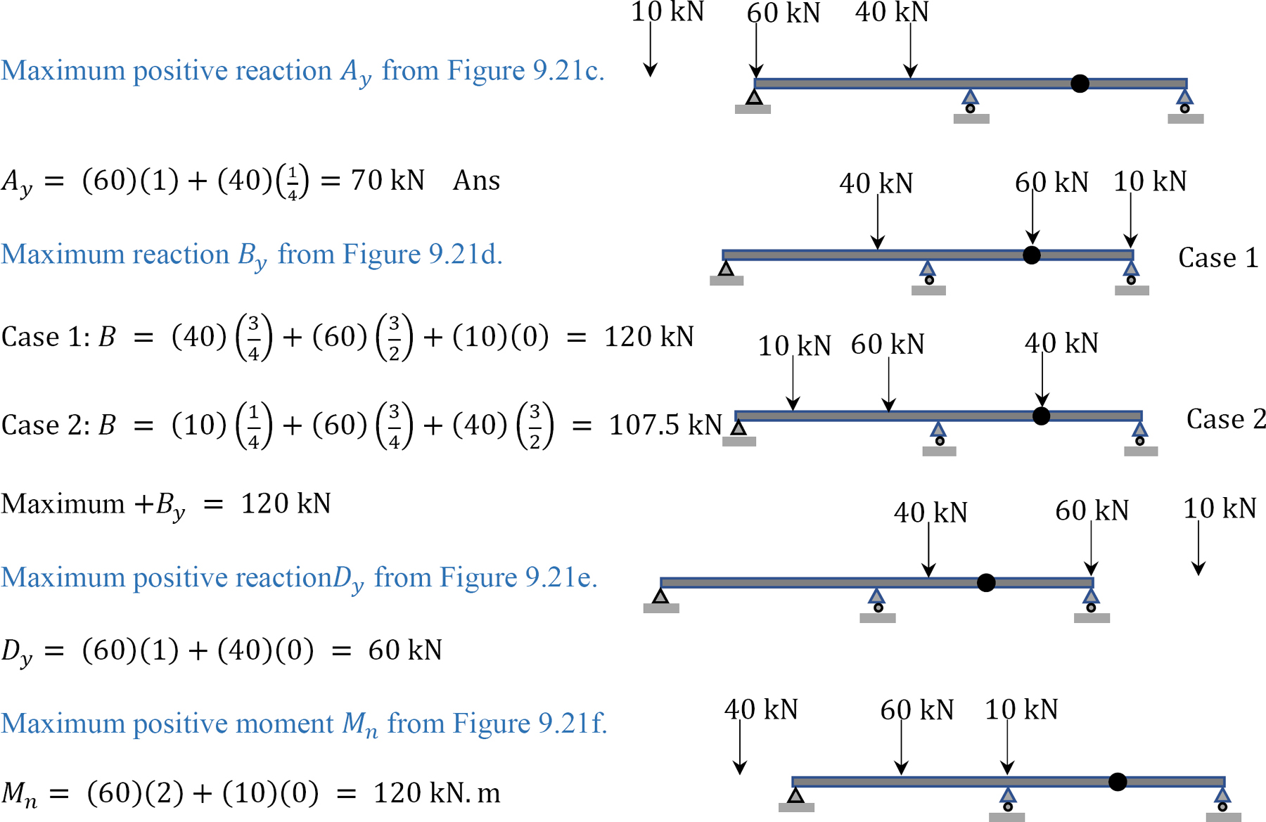
A compound beam shown in Figure 9.21a is subjected to a series of moving concentrated loads, which are shown in Figure 9.21b. Using influence lines, determine the magnitudes of the reactions at supports \(A\), \(B\), and \(C\) and the bending moment at section \(n\).

\(Fig. 9.21\). Compound beam.

Solution

Uses of Influence Lines to Determine Absolute Maximum Response Function at Any Point Along the Structure

The preceding sections explain the use of influence lines for the determination of the maximum response function that may occur at specific points of a structure. This section will explain the determination of the absolute maximum value of a response function that may occur at any point along the entire structure due to concentrated loads exerted by moving loads.

The absolute maximum shear force for a cantilever beam will occur at a point next to the fixed end, while that for a simply supported beam will occur close to one of its reactions. The absolute maximum moment for a cantilever beam will also occur close to the fixed end, while that for simply supported beam is not readily known and, thus, will require some analysis. To locate the position where the absolute maximum moment occurs in a simply supported beam, consider a beam subjected to three moving concentrated loads \(P_{1}\), \(P_{2}\), and \(P_{3}\), as shown in Figure 9.22.

Although it is certain from statics that the absolute maximum moment will occur under one of the concentrated loads, the specific load under which it will occur must be identified, and its location along the beam must be known. The concentrated load under which the absolute maximum moment will occur may be determined by inspection or by trial-and-error process, but the location of this load should be established analytically. Assume that the concentrated load under which the absolute maximum moment will occur is \(P_{3}\), and the distance of \(P_{3}\) from the centerline of the beam is \(x\). To obtain an expression for \(x\), first determine the resultant \(P_{R}\) of the concentrated loads, acting at a distance \(x^{\prime}\) from the load \(P_{3}\).

To determine the right reaction of the beam, take the moment about support \(A\), as follows:

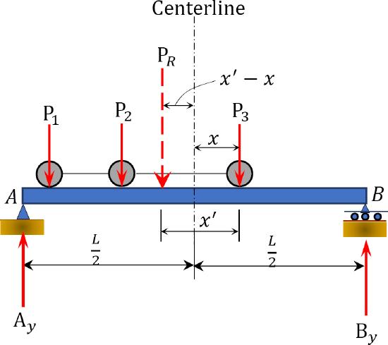
\(Fig. 9.22\). Beam subjected to three moving concentrated loads.

To determine the right reaction of the beam, take the moment about support \(A\), as follows:

\[\begin{aligned}
\sum M_{A} &=0 \\
B_{y} L &=P_{R}\left[\frac{L}{2}-\left(x^{\prime}-x\right)\right] \\
B_{y}=& \frac{P_{R}}{L}\left[\frac{L}{2}-\left(x^{\prime}-x\right)\right]
\end{aligned}\]

Thus, the bending moment under \(M_{3}\) is as follows:

\[\begin{aligned}
M_{3} &=B_{y}\left(\frac{L}{2}-x\right)=\frac{P_{R}}{L}\left[\frac{L}{2}-\left(x^{\prime}-x\right)\right]\left(\frac{L}{2}-x\right) \\
&=P_{R}\left(\frac{L}{4}-+\frac{x^{\prime}}{2}+\frac{x x^{\prime}}{L}-\frac{x^{2}}{L}\right)
\end{aligned}\]

The distance \(x\) for which \(M_{3}\) is maximum can be determined by differentiating equation 9.9 with respect to \(x\) and equating it to zero, as follows:

\(\begin{aligned}
\frac{d M_{3}}{d x} &=\mathrm{P}_{R}\left(\frac{x^{\prime}}{L}-\frac{2 x}{L}\right)=0 \\
\frac{2 x}{L} &=\frac{x^{\prime}}{L}
\end{aligned}\)

Therefore,

\[x=\frac{x^{\prime}}{2}\]

Equation 9.10 concludes that the absolute maximum moment in a simply supported beam occurs under one of the concentrated loads when the load under which the moment occurs and the resultant of the system of loads are equidistant from the center of the beam.

Example 9.14

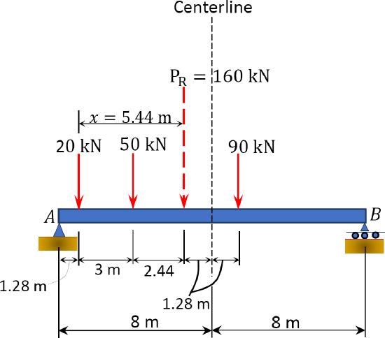
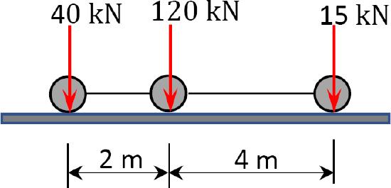
Determine the absolute maximum bending moment in a 16 m-long simply supported girder bridge subjected to a moving truck loading, as shown in Figure 9.23.

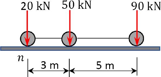
\(Fig. 9.23\). Simply supported girder beam.

Solution

Using statics, first determine the value and the position of the resultant of the moving loads.

Resultant load.

\(P_{R}=\sum P=20+50+90=160\)

Position of the resultant load. To determine the position of the resultant load, take the moment about point \(n\), which is directly below the 20 kN load, as follows:

\(\begin{aligned}
\sum M_{n}: 160 x &=(50)(3)+(90)(8) \\
x &=5.44 \mathrm{~m}
\end{aligned}\)

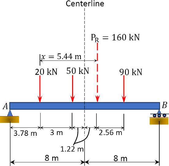
\(Fig. 9.24\). Resultant and load equidistant from centerline of the beam.

If the absolute maximum moment is assumed to occur under the 50 kN load, the positioning of the resultant and this load equidistant from the centerline of the beam is as shown in Figure 9.24. Before computing the absolute maximum moment, first determine the reaction \(B_{y}\) using statics.

\(\begin{aligned}
\sum M_{A} &=0:-(160)(9.22)+B_{y}(16)=0 \\
B_{y} &=92.2 \mathrm{kN}
\end{aligned}\)

The absolute maximum moment under the 50 kN load is as follows:

\(M_{50}=(92.2)(9.22)-(90)(3.78)=509.88 \mathrm{kN} \cdot \mathrm{m}\)

\(Fig. 9.25\). Resultant and load equidistant from centerline of the beam.

If the absolute maximum moment is assumed to occur under the 90 kN load, the positioning of the resultant and this load equidistant from the centerline of the beam will be as shown in Figure 9.25.

Before computing the absolute maximum moment, first determine the reaction \(B_{y}\) using statics.

\(\begin{array}{c}
\sum M_{A}=0:-(160)(6.72)+B_{y}(16)=0 \\
B_{y}=67.2 \mathrm{kN}
\end{array}\)

The absolute maximum moment under the 90 kN load is as follows:

\(M_{90}=(67.2)(6.72)=451.58 \mathrm{kN} \cdot \mathrm{m}\)

From the two possible cases considered in the solution, it is evident that the absolute maximum moment occurs under the 50 kN force.

Chapter Summary

Influence lines for statically determinate structures: The effect of a moving load on the magnitude of certain functions of a structure, such as support reactions, deflection, and shear force and moment, at a section of the structure vary with the position of the moving load. Influence lines are used to study the maximum effect of a moving load on these functions for design purposes. The influence lines for determinate structures can be obtained by the static equilibrium method or by the kinematic or Muller-Breslau method. The influence lines by the former method can be determined quantitatively, while those for the latter method can be obtained qualitatively, as have been demonstrated in this chapter. Several example problems are solved showing how to construct the influence lines for beams and trusses using the afore-stated methods.

Practice Problems

9.1 Draw the influence line for the shear force and moment at a section n at the midspan of the simply supported beam shown in Figure P9.1.

\(Fig. P9.1\). Simply supported beam.

9.2 Draw the influence lines for the reaction at \(A\) and \(B\) and the shear and the bending moment at point \(C\) of the beam with overhanging ends, as shown in Figure P9.2.

\(Fig. P9.2\). Beam with overhang.

9.3 Draw the influence line for the reactions at the support of the cantilever beam shown in Figure P9.3.

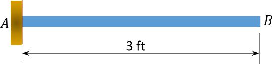
\(Fig. P9.3\). Cantilever beam.

9.4 Draw the influence line for the support reactions at \(B\) and \(D\) and shear and bending moments at section \(n\) of the beam shown in Figure 9.4.

\(Fig. P9.4\). Beam

9.5 Draw the influence lines for support reactions at \(C\) and \(D\) and at point \(B\) of the compound beam shown in Figure P9.5.

\(Fig. P9.5\). Compound beam.

9.6 Draw the influence lines for the shear force and moment at sections \(n, s\) and \(k\) of the compound beam shown in Figure P9.6.

\(Fig. P9.6\). Compound beam.

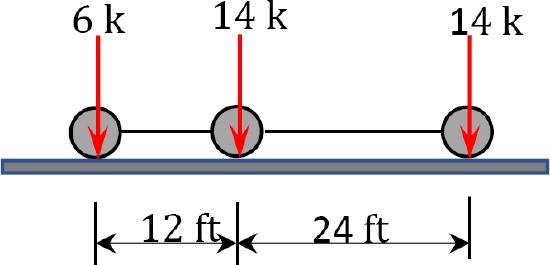
9.7 Determine the absolute maximum bending moment in a 65 ft-long simply supported girder bridge subjected to a moving truck loading, as shown in Figure P9.7.

\(Fig. P9.7\). Simply supported girder bridge.

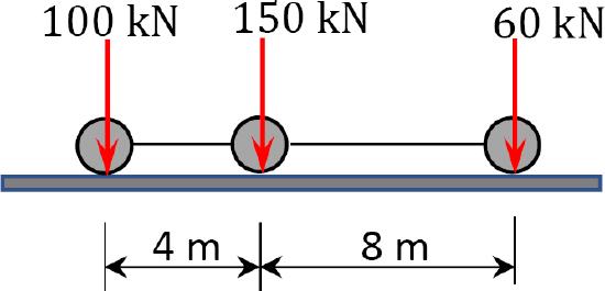
9.8 Determine the absolute maximum bending moment in a 12 m-long simply supported girder bridge subjected to a moving truck loading, as shown in Figure P9.8.

\(Fig. P9.8\). Simply supported girder bridge.

9.9 Determine the absolute maximum bending moment in a 40 ft-long simply supported girder bridge subjected to a moving truck loading, as shown in Figure P9.9.

\(Fig. P9.9\). Simply supported girder bridge.

9.10 Determine the absolute maximum bending moment in a 14 m-long simply supported girder bridge subjected to a moving truck loading, as shown in Figure P9.10.

\(Fig. P9.10\). Simply supported girder bridge.

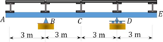
9.11 Draw the influence lines for the moment at \(B\) and the shear force in panel \(CD\) of the floor girder shown in Figure P9.11.

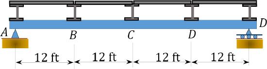
\(Fig. P9.11\). Floor girder.

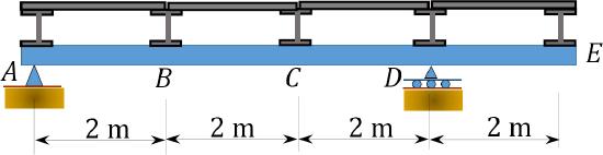
9.12 Draw the influence lines for the moment at \(C\) and the shear force in panel \(BC\) of the floor girder shown in Figure P9.12.

\(Fig. P9.12\). Floor girder.

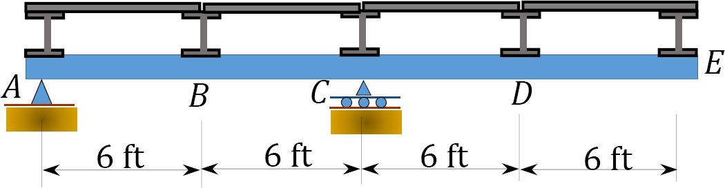
9.13 Draw the influence lines for the moment at \(B\) and the shear in panel \(CD\) of the floor girder shown in Figure P9.13.

\(Fig. P9.13\). Floor girder.

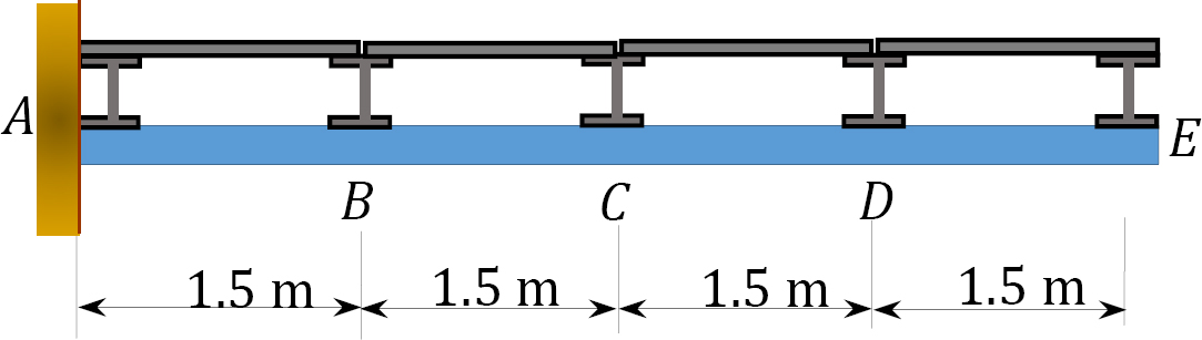
9.14 Draw the influence lines for the moment at \(D\) and the shear force in panel \(DE\) of the floor girder shown in Figure P9.14.

\(Fig. P9.14\). Floor girder.

9.15 Draw the influence lines for the moment at \(D\) and the shear force in panel \(AB\) of the floor girder shown in Figure P9.15.

\(Fig. P9.15\). Floor girder.

9.16 Draw the influence lines for the forces in members \(CD\), \(CF\), and \(GF\) as a unit load moves across the top of the truss, as shown in Figure P9.16.

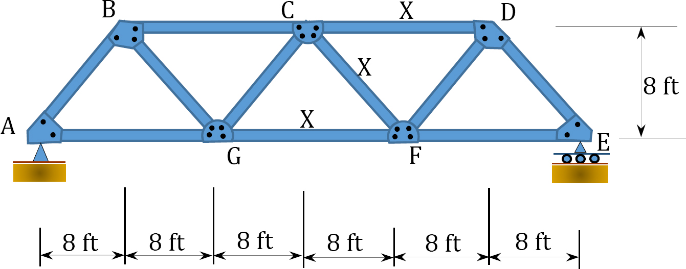
\(Fig. P9.16\). Truss.

9.17 Draw the influence lines for the forces in members \(DE\), \(NE\), and \(NM\) as a unit live load is transmitted to the top chords of the truss, as shown in Figure P9.17.

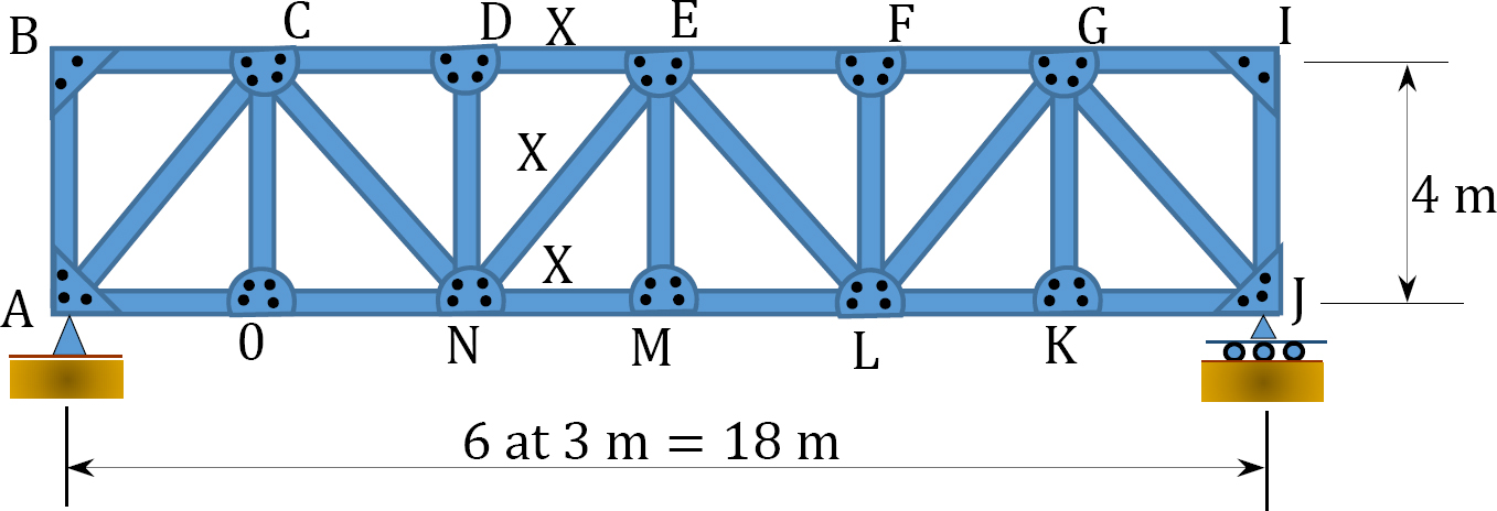
\(Fig. P9.17\). Truss.

9.18 Draw the influence lines for the forces in members \(DE\), \(DH\), \(IH\), and \(HG\) as a unit live load is transmitted to the bottom chords of the truss, as shown in Figure P9.18.

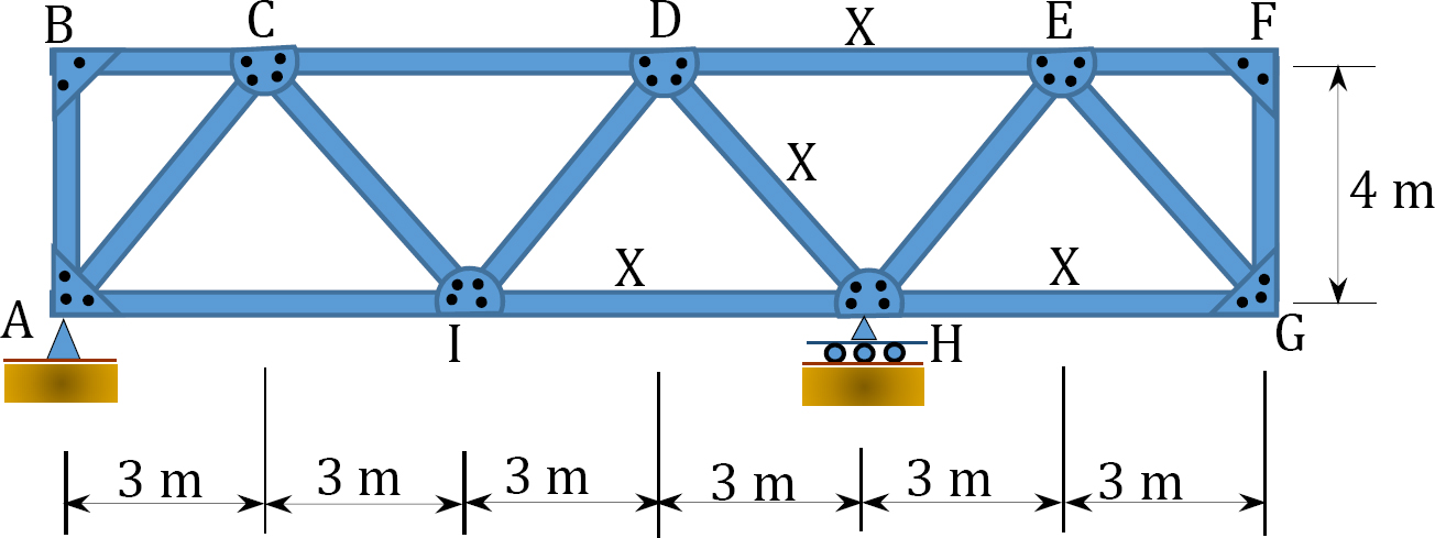
\(Fig. P9.18\). Truss.

9.19 Draw the influence lines for the forces in members \(BC\), \(BF\), \(FE\), and \(ED\) as a unit load moves across the bottom chords of the truss, as shown in Figure P9.19.

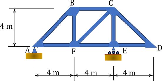
\(Fig. P9.19\). Truss.