9.3: Construction of Influence Lines

In practice, influence lines are mostly constructed, and the values of the functions are determined by geometry. The procedure for the construction of influence lines for simple beams, compound beams, and trusses will be outlined below and followed by a solved example to clarify the problem. For each case, one example will be solved immediately after the outline.

Simple Beams Supported at Their Ends

The procedures for the construction of the influence lines (I.L.) for some functions of a beam supported at both ends are as follows:

9.3.1.1 Influence Line for Left End Support Reaction, \(R_{A}\) (Fig. 9.2)

(a)At the position of the left end support (point \(A\)), along the y-axis, plot a value +1 (point \(A^{\prime}\)).

 

(b)Draw a line joining point \(A^{\prime}\) and the zero ordinate at point \(B\). Point \(B\) is at the position of support \(B\).

 

(c)The triangle \(AA^{\prime}B\) is the influence line for the left-end support reaction. The idea here is that when the unit load moves across the beam, its maximum effect on the left-end reaction will be when it is directly lying on the left end support. As the load moves away from the left end support, its influence on the left end reaction will continue to diminish until it gets to the least value of zero, when it is lying directly on the right end support.

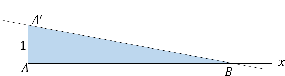
\(Fig. 9.2\). Influence line for \(R_{A}\).

9.3.1.2 Influence Line for Right End Support Reaction \(R_{B}\) (Fig. 9.3)

(a)At the right end support (point \(B\)), plot an ordinate of value +1 (point \(B^{\prime}\)).

 

(b)Draw a line joining point \(B^{\prime}\) and point \(A\).

 

(c)The triangle \(AB^{\prime}B\) is the influence line for the right end support reaction. The explanation for the influence line for the right end support reaction is similar to that given for the left end support reaction. The maximum effect of the unit load occurs when it is lying directly on the right support. As the load moves away from the right end support, its influence on the support reaction decreases until it is zero, when the load is directly lying on the left support.

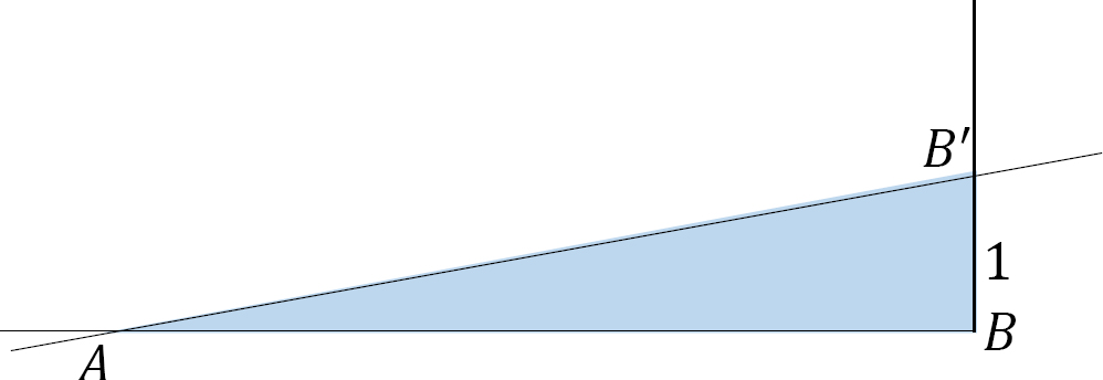
\(Fig. 9.3\). Influence line for \(R_{B}\).

9.3.1.3 Influence Line for Shearing Force at Section \(n\)

(a) At the left end support (point \(A\)), plot an ordinate equal +1 (point \(A^{\prime}\)), as shown in Figure 9.4b.

 

(b) Draw a line joining point \(A^{\prime}\) and the zero ordinate at point \(B\).

 

(c) At the right end support (point \(B\)), plot an ordinate equal –1 (point \(B^{\prime}\)).

 

(d) Draw a line joining \(B^{\prime}\) and the zero ordinate at point \(A\).

 

(e) Drop a vertical line from the section under consideration to cut lines \(A^{\prime}B\) and \(AB^{\prime}\) at points \(N^{\prime}\) and \(N^{\prime \prime\), respectively.

 

(f) The diagram ABN′N″ is the influence line of the shear force at the section n.

 

(g) Use a similar triangle to determine the ordinates n-N’ and n-N,” as follows:

\(\begin{array}{l}
\frac{1}{L}=\frac{n-N^{\prime}}{b} \rightarrow N^{\prime}=\frac{b}{L} \\
\frac{-1}{L}=\frac{n-N^{\prime \prime}}{a} \rightarrow N^{\prime \prime}=-\frac{a}{L}
\end{array}\)

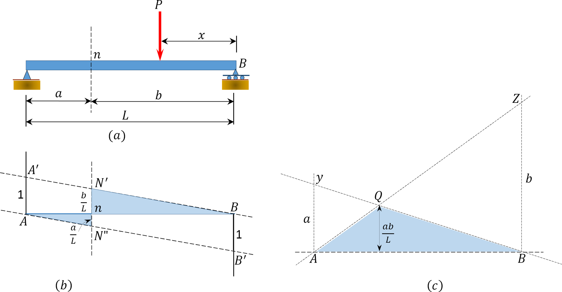
\(Fig. 9.4\). Influence line for shear (\(b\)) and moment (\(c\)) at section \(m\).

9.3.1.4 Influence Line for Bending Moment at Section \(n\)

(a) At the left end support (point \(A\)), plot an ordinate of a value equal to the distance from the left end support to the section \(n\). For example, the distance \(a\) in Figure 9.4c (denoted as point \(Y\) in Figure 9.4c).

 

(b) Draw a line joining point \(Y\) and the zero ordinate at point \(B\) at the right end support.

 

(c) Draw a vertical line passing through section \(n\) and intersecting the line \(AZ\) at point \(Q\).

 

(d) Draw a straight line \(AQ\) connecting \(A\) and \(Q\).

 

(e) The triangle \(AQB\) is the influence line for the moment at section \(n\). Alternatively, ignore steps (b), and (c) and (d) and go to step (f).

 

(f) At the right end support (point \(B\)), plot an ordinate equal +b. For example, the distance from the right end support to the section \(n\) (denoted as point \(Z\)).

 

(g) Draw a line joining \(Z\) and the zero ordinate at \(A\) (position of the left end support).

 

(h) At the left end support (point \(A\)), plot an ordinate equal +a. For example, the distance from the left end support to the section \(n\) (denoted point \(Y\)).

 

(i) Draw a line joining \(Y\) and the zero ordinate at \(B\) (position of the right end support).

 

(j) Lines \(AZ\) and \(BY\) intersect at \(Q\).

 

(k) The triangle \(AQB\) is the influence line for the moment at section \(n\). If accurately drawn, with the right sense of proportionality, the intersection \(Q\) should lie directly on a vertical line passing through the section \(n\).

 

(l) The value of the ordinate \(nQ\) can be obtained using a similar triangle, as follows:

\(\begin{array}{l}
\frac{a}{L}=\frac{n Q}{b} \rightarrow n Q=\frac{a b}{L} \\
\text { or } \frac{b}{L}=\frac{n Q}{a} \rightarrow n Q=\frac{a b}{L}
\end{array}\)

Example 9.1

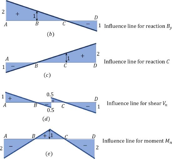
For the double overhanging beam shown in Figure 9.5a, construct the influence lines for the support reactions at \(B\) and \(C\) and the shearing force and the bending moment at section \(n\).

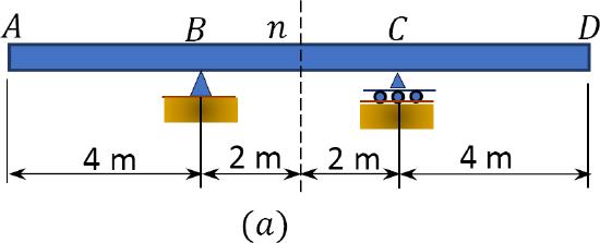
\(Fig. 9.5\). Double overhanging beam.

Solution

I.L. for \(B_{y}\)_.

Step 1. At the position of support \(B\) (point \(B\)), plot an ordinate +1.

Step 2. Draw a straight line connecting the plotted point (+1) to the zero ordinate at the position of support \(C\).

Step 3. Continue the straight line in step 2 until the end of the overhangs at both ends of the beam. The influence line for \(B_{y}\) is shown in Figure 9.5b.

Step 4. Determine the ordinates of the influence line at the overhanging ends using a similar triangle, as follows:

Ordinate at \(A\):

\(\frac{1}{B C}=\frac{x}{A C} ; \Rightarrow x=\frac{A C}{B C}=\frac{8}{4}=2 \mathrm{~m}\)

Ordinate at \(D\):

\(\frac{1}{B C}=\frac{x}{C D} ; \Rightarrow x=\frac{C D}{B C}=\frac{4}{4}=1 \mathrm{~m}\)

I.L. for \(C_{y}\)_.

Step 1. At the position of support \(C\) (point \(C\)), plot an ordinate +1.

Step 2. Draw a straight line connecting the plotted point (+1) to the zero ordinate at the position of support \(B\).

Step 3. Continue the straight line in step 2 until the end of the overhangs at both ends of the beam. The influence line for \(B_{y}\) is shown in Figure 9.5c.

Step 4. Determine the ordinates of the influence line at the overhanging ends using a similar triangle, as follows:

Ordinate at \(D\):

\(\frac{1}{B C}=\frac{x}{B D} ; \Rightarrow x=\frac{B D}{B C}=\frac{8}{4}=2 \mathrm{~m}\)

Ordinate at \(A\):

\(\frac{x}{A B}=\frac{1}{B C} ; \Rightarrow x=\frac{A B}{B C}=\frac{4}{4}=1 \mathrm{~m}\),

I.L. for shear \(V_{n}\).

Step 1. At the position of support \(B\) (point \(B\)), plot an ordinate +1.

Step 2. Draw a straight line connecting the plotted point (+1) to the zero ordinate at the position of support \(C\). Continue the straight line at \(C\) until the end of the overhang at end \(D\).

Step 3. At the position of support \(C\) (point \(C\)), plot an ordinate –1.

Step 4. Draw a straight line connecting the plotted point (–1) to the zero ordinate at the position of support \(B\). Continue the straight line at \(B\) until the end of the overhang at end \(A\).

Step 5. Draw a vertical passing through the section whose shear is required to intersect the lines in step 2 and step 3.

Step 6. Connect the intersections to obtain the influence line, as shown in Figure 9.5d.

Step 7. Determine the ordinates of the influence lines at other points by using similar triangles, as previously demonstrated.

I.L. for Moment \(M_{n}\)_.

Step 1. At point \(B\), plot the ordinate equal +2 m.

Step 2. Draw a straight line connecting the plotted ordinate in step 1 to the zero ordinate in support \(C\).

Step 3. At point \(C\), plot the ordinate equal +2 m.

Step 4. Draw a straight line connecting the plotted ordinate in step 3 to the zero ordinate at support \(B\).

Step 5. Continue the straight lines from the intersection of the lines drawn in steps 2 and 4 through the supports to the overhanging ends, as shown in Figure 9.5e.

Step 6. Determine the values of the influence lines at other points using similar triangles, as previously demonstrated.

Example 9.2

For the beam with one end overhanging support B, as shown in Figure 9.6, construct the influence lines for the bending moment at support \(B\), the shear force at support \(B\), the support reactions at \(B\) and \(C\), and the shearing force and the bending moment at a section “\(k\).”

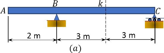
\(Fig. 9.6\). Beam with one overhanging support.

Solution

The influence lines in example 9.2 for the desired functions were constructed based on the procedure described in the previous section and example.

Compound Beams

To correctly draw the influence line for any function in a compound beam, a good understanding of the interaction of the members of the beam is necessary, as was discussed in chapter 3, section 3.3. The student should recall from the previous section that a compound beam is made up of the primary structure and the complimentary structure. The two facts stated below must always be remembered, since the extent of the spread of the influence line of compound beams depends on them. Remembering these facts will also serve as a temporary check to ascertain the correctness of the drawn influence line.

The moving unit load will have an effect on the functions of the primary structure when it is located at any point, not only on the primary structure but also on the complimentary structure, since the latter constitutes a loading on the former.

The moving unit load will have effect only on the functions of the complimentary structure when it is located within the complimentary structure; it will not have an effect on any function of the complimentary structure when it is at any point on the primary structure.

The afore-stated facts will be demonstrated in the following examples.

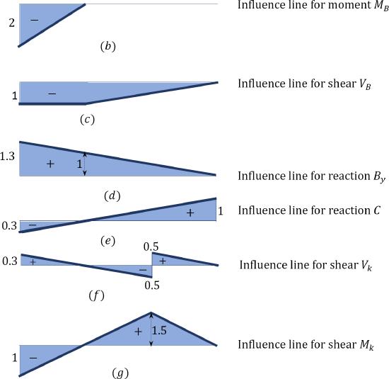
Example 9.3

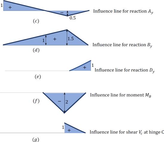
For the compound beam shown in Figure 9.7, construct the influence lines and indicate the critical ordinates for the support reactions at \(A\), \(B\), and \(D\), the bending moment at \(B\), and the shear at hinge \(C\).

\(Fig. 9.7\). Compound beam.

Solution

Prior to the construction of the influence lines for desired functions, it is necessary to first observe the extent of the influence lines through the schematic diagram of member-interaction, as shown in Figure 9.7b.

I.L. for \(A_{y}\). The reaction \(A_{y}\) is a function in the primary structure, so the unit load will have influence on this function when it is located at any point on the beam, as was previously stated in section 9.3.2. With this understanding, construct the influence line of \(A_{y}\), as follows:

Step 1. At point \(A\), plot an ordinate +1.

Step 2. Draw a straight line connecting the plotted ordinate in step 1 to the zero ordinate in support \(B\) and continue this line until the end of the overhanging end of the primary structure, as shown in the interaction diagram.

Step 3. Draw a straight line connecting the ordinate at the end of the overhang to the zero ordinate at support \(D\). The influence line is as shown in Figure 9.7c.

Step 4. Use a similar triangle to compute the ordinates of the influence line

I.L. for \(B_{y}\). The influence line for this reaction will cover the entire length of the beam because it is a support reaction in the primary structure. With this knowledge, construct the influence line for \(B_{y}\), as follows:

Step 1: At point \(B\), plot an ordinate +1.

Step 2. Draw a straight line connecting the plotted ordinate in step 1 to the zero ordinate in support \(A\). Continue the line in support \(B\) until the end of the overhanging end of the primary structure, as shown in the interaction diagram.

Step 3. Draw a straight line connecting the ordinate at the overhanging end to the zero ordinate at support \(D\). The influence line for \(B_{y}\) is shown in Figure 9.7d.

Step 4. Use a similar triangle to determine the values of the ordinate of the influence line.

I.L. for \(D_{y}\). The reaction \(D_{y}\) is a function in the complimentary structure and will be influenced when the unit load lies at any point along the complimentary structure. It will not be influenced when the unit load transverses the primary structure, as was stated in section 9.3.2. Thus, the extent of the influence line will be the length of the complimentary structure. Knowing this, draw the influence line for \(D_{y}\).

Step 1. At point \(D\), plot the ordinate +1.

Step 2. Draw a straight line connecting the plotted ordinate in step 1 to the zero ordinate at hinge \(C\). The influence line for \(D_{y}\) is as shown in Figure 9.7e.

The influence lines for the moment at \(B\) and the shear \(C\) are shown in Figure 9.7f and Figure 9.7g, respectively.

Example 9.4

For the compound beam shown in Figure 9.8a, construct the influence lines and indicate the critical ordinates for the support reactions at \(F\) and \(G\), the shear force and bending moment at \(D\), and the moment at \(F\).

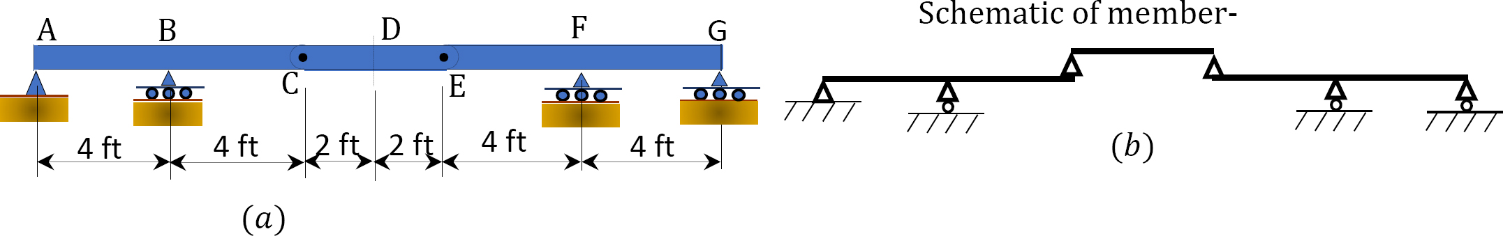
\(Fig. 9.8\). Compound beam.

Solution

Shown in Figure 9.8c through Figure 9.8g are the influence lines for the desired functions. The schematic diagram of the member interaction shown in Figure 9.8b immeasurably aids the initial perception of the range of the influence line of each function. Construction of the influence lines follows the description outlined in the previous sections.

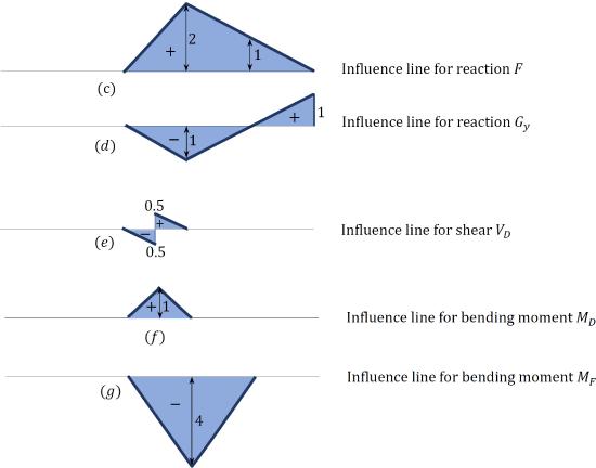
Influence Lines for Girders Supporting Floor Systems

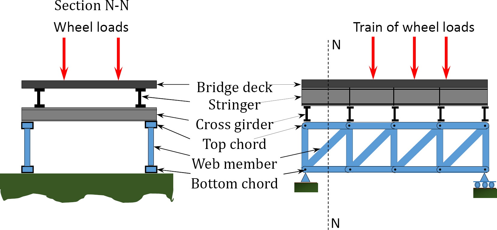
Thus far, the examples and text have only considered cases where the moving unit load is applied directly to the structure. But, in practice, this may not always be the case. For instance, sometimes loads from building floors or bridge decks are transmitted through secondary beams, such as stringers and cross beams to girders supporting the building or bridge floor system, as shown in Figure 9.9. Columns, piers, or abutments in turn support the girders.

\(Fig. 9.9\). Transfer of load to girder by system of stringers and floor beams.

 

\(Fig. 9.10\). Influence lines in a case of indirect application of loads.

Example 9.5

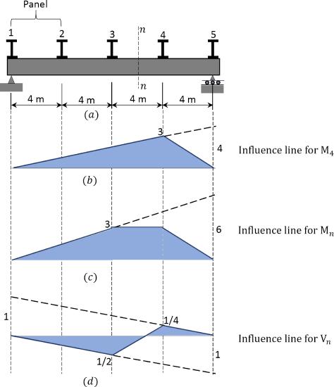
Draw the influence lines for the moment at \(C\) and the shear in panel \(BC\) of the floor girder shown in Figure 9.11.

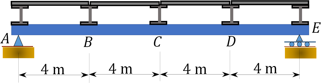
\(Fig. 9.11a\). Floor girder.

Solution

Influence line for \(M_{c}\). To obtain the values of the influence line of \(M_{c}\), successively locate a load of 1 kN at panel points \(A\), \(B\), \(C\), \(D\), and \(E\). To determine the moment, use the equation of statics. The values of \(M_{c}\) at the respective panel points are presented in Table 9.1. When the unit load is located at \(B\), as shown in Figure 9.11b, the value of \(M_{c}\) is determined as follows:

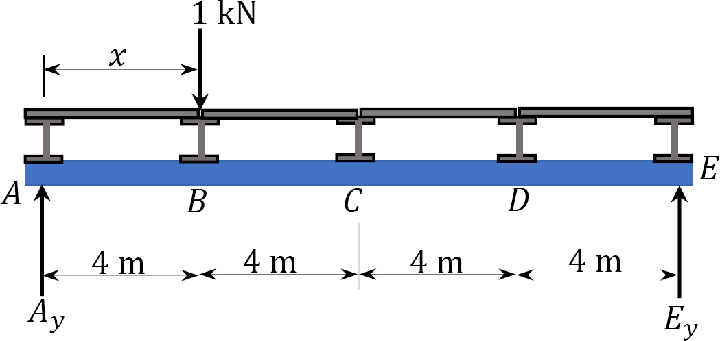
\(Fig. 9.11b\). Unit load at \(B\).

First, determine the support reactions in the beam using the equation of static equilibrium.

\(\begin{array}{lll}
+\cup \sum M_{E}=0 & -A_{y}(16)+1(12)=0 & A_{y}=0.75 \mathrm{kN} \\
+\uparrow \sum F_{y}=0 & 0.75+E_{y}-1=0 & E_{y}=0.25 \mathrm{kN}
\end{array}\)

Then, using the computed reaction, determine \(M_{c}\), as follows:

\(M_{c}=0.25(12)=3 \mathrm{kN}-\mathrm{m}\)

\(Table 9.1\). The values of \(M_{c}\) at the respective panel points.

x(m)	Reactions (kN)		MC(kN.m)
	Ay	Ey
0 4 8 12 16	1 0.75 0.5 0.25 0	0 0.25 0.5 0.75 1	0 0.25(8)=2 0.5(8)=4 0.25(8)=2 0

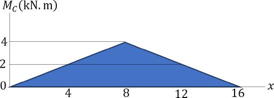
\(Fig. 9.11c\). Influence line for \(M_{c}\).

Influence line for \(V_{BC}\). To obtain the values of the influence line of \(MV_{BC}\), a load of 1 kN is successively located at panel points \(A\), \(B\), \(C\), \(D\), and \(E\). To determine the shear force, use the equation of statics. The values of \(V_{C}\) at the respective panel points are presented in Table 9.2.

\(Table 9.2\). The values of \(V_{C}\) at the respective panel points.

x(m)	Reactions (kN)		VBC(kN)
	Ay	Ey
0 4 8 12 16	1 0.75 0.5 0.25 0	0 0.25 0.5 0.75 1	0 -0.25 0.5 0.25 0

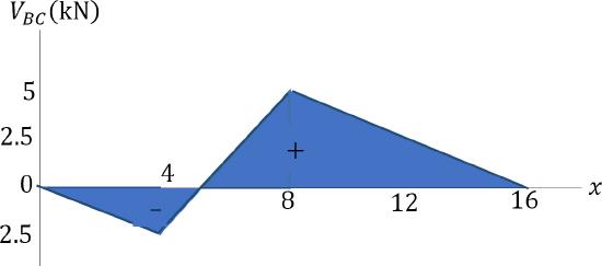
\(Fig. 9.11d\). Influence line for V_BC.

Influence Lines for Trusses

The procedure for the construction of influence lines for truss members is similar to that of a girder supporting a floor system considered in section 9.3.3. Loads can be transmitted to truss members via the top or bottom panel nodes. In Figure 9.12 the load is transmitted to members through the top panel nodes. As the live loads move across the truss, they are transferred to the top panel nodes by cross beams and stringers. The influence lines for axial forces in truss members can be constructed by connecting the influence line ordinates at the panel nodes with straight lines.

\(Fig. 9.12\). Load transferred by system of stringers and cross beams.

To illustrate the procedure for the construction of influence lines for trusses, consider the following examples.

Example 9.6

Draw the influence lines for the reactions \(A_{y}\), \(F_{y}\), and for axial forces in members \(CD\), \(HG\), and \(CG\) as a unit load moves across the top of the truss, as shown in Figure 9.13.

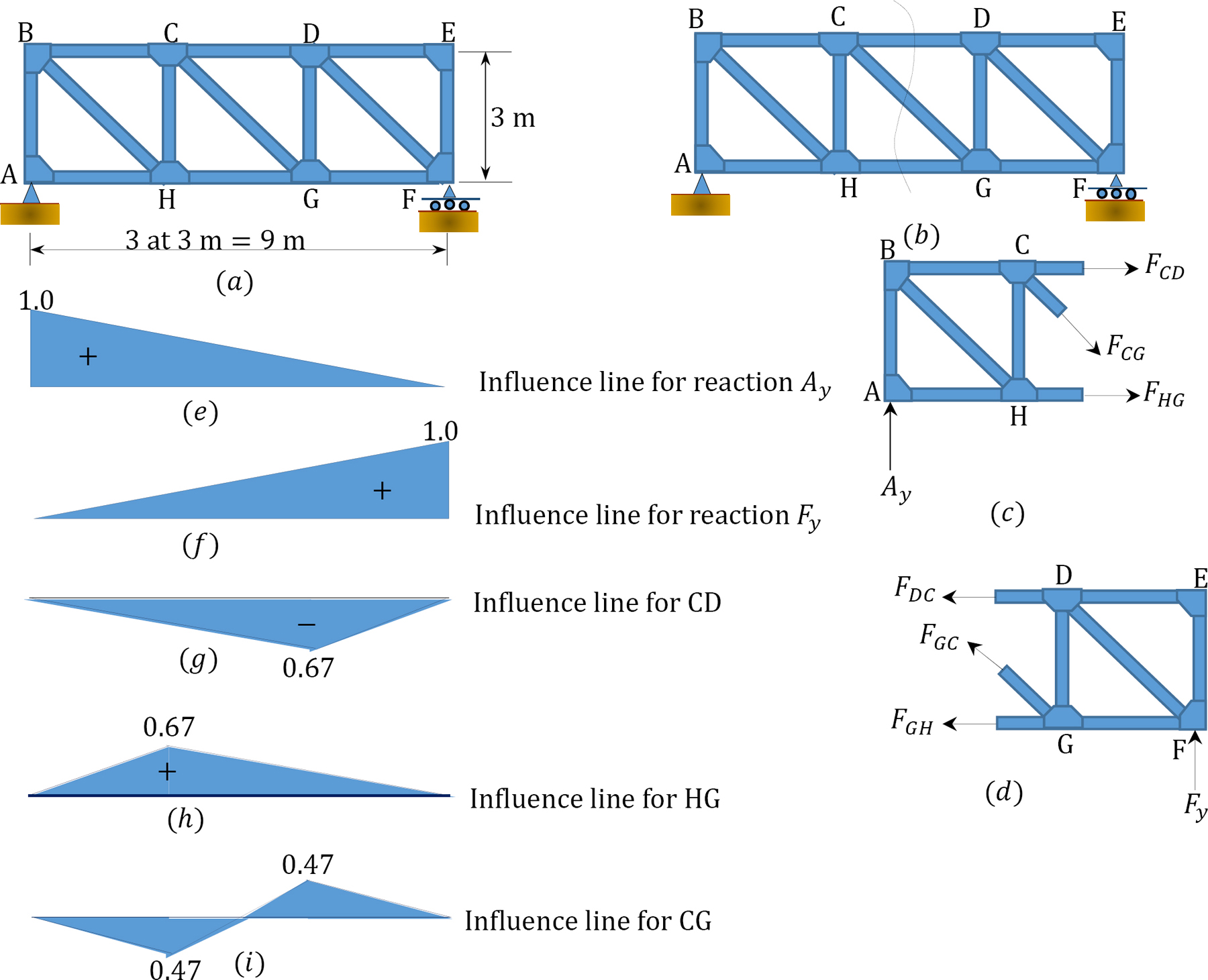
\(Fig. 9.13\). Truss.

Solution

The drawing of the influence lines for trusses is similar to that of a beam. The first step towards drawing the influence lines for the axial forces in the stated members is to pass an imaginary section through the members, as shown in Figure 9.13b, and to apply equilibrium to the part on either side of the section. The step-by-step procedure for drawing the influence line for each of the members is stated below.

Influence line for the axial force in member \(CD\). When the unit load is situated at any point to the right of \(D\), considering the equilibrium of the left segment \(AH\) (Fig. 9.13c), it suggests the following:

 

The obtained expression of \(F_{CD}\) in terms of \(A_{y}\) is indicative of the fact that the influence line for \(F_{CD}\) in the portion \(DE\) can be determined by multiplying the corresponding portion of the influence line for the reaction \(A_{y}\) by – 2. The influence line for \(A_{y}\) is shown in Figure 9.13e.

When the unit load is situated at any point to the left of \(C\), considering the equilibrium of the right segment \(GF\) (Fig. 9.13d), it suggests the following:

\(+v \sum M_{G}=0 \quad F_{y}(3)+F_{C D}(3)=0 \quad F_{C D}=-F_{y}\)

The obtained expression of \(F_{CD}\) in terms of \(F_{y}\) is indicative of the fact that the influence line for \(F_{CD}\) in the portion \(AH\) can be determined by multiplying the corresponding portion of the influence line for the reaction \(F_{y}\) by – 1. The influence line for \(F_{y}\) is shown in Figure 9.13f.

The influence line of the axial force in member \(CD\) constructed from the influence lines for the reactions \(A_{y}\) and \(F_{y}\) is shown in Figure 9.13g.

Influence line for member \(HG\). When the unit load is situated at any point to the right of \(D\), considering the equilibrium of the left segment \(AH\) (Fig. 9.13c), it suggests the following:

\(+v \sum M_{c}=0 \quad-A_{y}(3)+F_{H G}(3)=0 \quad F_{H G}=A_{y}\)

The obtained expression of \(F_{HG}\) in terms of \(A_{y}\) implies that the influence line for \(F_{HG}\) in the portion \(DE\) is identical to that of \(A_{y}\) within the corresponding segment.

When the unit load is situated at any point to the left of \(C\), considering the equilibrium of the right segment \(GF\) (Fig. 9.13d), it suggests the following:

\(+\cup \sum M_{c}=0 \quad F_{y}(6)-F_{H G}(3)=0 \quad F_{H G}=2 F_{y}\)

The obtained expression of \(F_{HG}\) in terms of \(F_{y}\) is indicative of the fact that the influence line for \(F_{HG}\) in the portion \(AH\) can be determined by multiplying the corresponding portion of the influence line for the reaction \(F_{y}\) by 2.

The influence line of the axial force in member \(HG\) constructed from the influence line for the reactions \(A_{y}\) and \(F_{y}\) is also shown in Figure 9.13h.

Influence line for the axial force in member \(CG\). When the unit load is situated at any point to the right of \(D\), considering the equilibrium of the left segment \(AH\) (Fig. 9.13C), it suggests the following:

\(\begin{array}{rl}
+\uparrow \sum F_{y}=0 & A_{y}-F_{C G} \cos 45^{\circ}=0 \\
F_{C G} & =\frac{A y}{\cos 45^{\circ}}=1.41 A_{y}
\end{array}\)

The obtained expression of \(F_{CG}\), with reference to \(A_{y}\), implies that the influence line for \(F_{CG}\) in the portion \(DE\) can be determined by multiplying the corresponding portion of the influence line for the reaction \(A_{y}\) by 1.41.

When the unit load is situated at any point to the left of \(C\), considering the equilibrium of the right segment \(GF\) (Fig. 9.13d), it suggests the following:

\(\begin{aligned}
F_{y}+F_{C G} \cos 45^{\circ} &=0 \\
F_{C G} &=-\frac{F_{y}}{\cos 45^{\circ}}=-1.41 F_{y}
\end{aligned}\)

The obtained expression of \(F_{CG}\) in terms of \(F_{y}\) is indicative of the fact that the influence line for \(F_{CG}\) in the portion \(AH\) can be determined by multiplying the corresponding portion of the influence line for the reaction \(F_{y}\) by – 1.41.

The influence line of the axial force in member \(CG\) constructed from the influence line for the reactions \(A_{y}\) and \(F_{y}\) is shown in Figure 9.13i.

Example 9.7

Draw the influence lines for the force in member \(CH\) as a unit load moves across the top of the truss, as shown in Figure 9.14a.

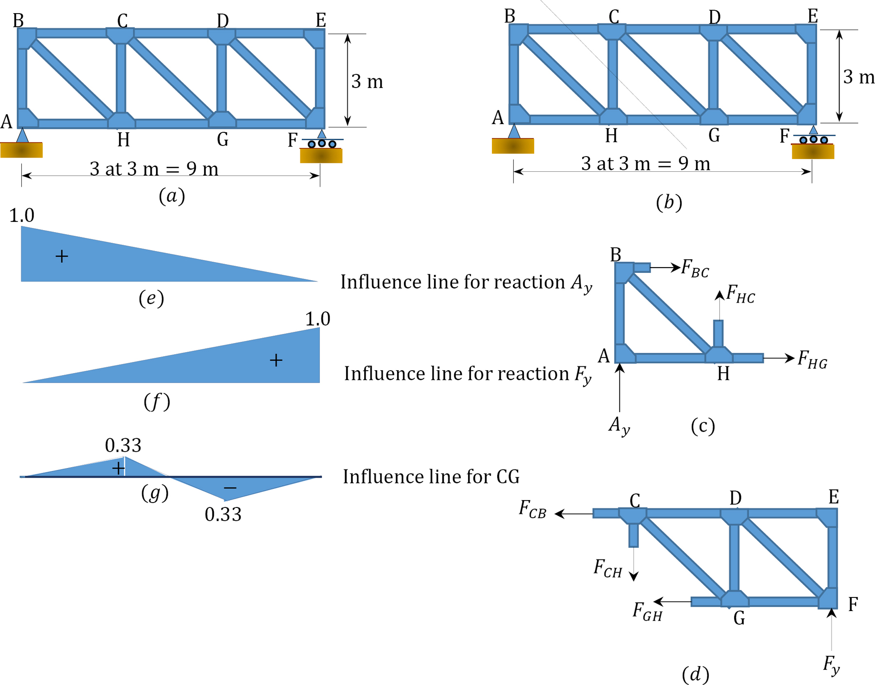
\(Fig. 9.14\). Truss.

Solution

To obtain the expression for the influence line for the axial force in member \(CH\), first pass an imaginary section that cuts through this member, as shown in Figure 9.14a.

When the unit load is situated at any point to the right of \(G\), considering the equilibrium of the left segment \(AH\) (Fig. 9.14 C), it suggests the following:

\(\begin{array}{rlrl}
+\uparrow \sum F_{y}=0 & A_{y}+F_{C H} & =0 \\
F_{C H} & =-A_{y}
\end{array}\)

The obtained expression of \(F_{CH}\) in terms of \(A_{y}\) indicates that the influence line for \(F_{CH}\) in the portion \(AH\) can be determined by multiplying the corresponding portion of the influence line for the reaction \(A_{y}\) by – 1.

When the unit load is located at any point to the left of \(H\), considering the equilibrium of the right segment \(GF\) (Fig. 9.14d), it suggests the following:

\(+\uparrow \sum F_{y}=0 \quad \begin{array}{c}
F_{y}-F_{C H}=0 \\
F_{C H}=F_{y}
\end{array}\)

The obtained expression of \(F_{CH}\) in terms of \(F_{y}\) implies that the influence line for \(F_{CH}\) in the portion \(GF\) is identical to that of \(F_{y}\) within the corresponding segment.

The influence line of \(CG\) is shown in Figure 9.14g.