10.3: Analysis of Indeterminate Beams and Frames

The analyses of indeterminate beams and frames follow the general procedure described previously. First, the primary structures and the redundant unknowns are selected, then the compatibility equations are formulated, depending on the number of the unknowns, and solved. There are several methods of computation of flexibility coefficients when analyzing indeterminate beams and frames. These methods include the use of the Mohr integral, deflection tables, and the graph multiplication method. These methods are illustrated in the solved example problems in this section.

Computation of Flexibility Coefficients Using the Mohr Integral

The Mohr integral for obtaining the flexibility coefficient for beams and frames is expressed as follows: \[\begin{array}{l}
\Delta_{B P}=\int \frac{M m}{E I} d x \\
\delta_{B B}=\int \frac{m^{2}}{E I} d x \\
\theta_{A P}=\int \frac{M m_{\theta}}{E I} d x \\
\alpha_{A A}=\int \frac{m_{\theta}^{2}}{E I} d x
\end{array}\]

where

• \(M\) = moment in the primary structure due to the applied load \(P\).
• \(m\) = moment in the primary structure due to a unit load applied at \(B\).
• \(m_{\theta}\) = moment in the primary structure due to a unit moment applied at \(A\).

Example \(\PageIndex{1}\)

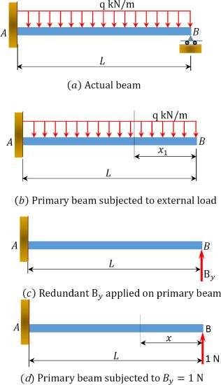
Determine the reactions in the beam shown in Figure 10.3a. Use the method of consistent deformation to carry out the analysis. All flexibility coefficients are determined by integration. \(EI\) = constant.

\(Fig. 10.3\). Beam.

Solution

Classification of structure. There are four unknown reactions in the beam: three unknown reactions at the fixed end \(A\) and one unknown reaction at the prop \(B\). Since there are three equations of equilibrium on a plane, it implies that the beam has one unknown reaction in excess of the equations of equilibrium on a plane, thus it is indeterminate to one degree.

Choice of primary structure. There may be more than one possible choice of primary structure. For the given propped cantilever beam, the prop at \(B\) will be selected as the redundant. Thus, the primary structure is as shown in Figure 10.3b.

Compatibility equation. The number of compatibility equations will always match the number of the redundant reactions in a given structure. For the given cantilever beam, the number of compatibility equations is one and is written as follows:

\(\Delta_{B P}+B_{y} \delta_{B B}=0\)

The flexibility or compatibility coefficients \(\Delta_{B P}\) and \(\delta_{B B}\) can be computed by several methods, including the integration method, the graph multiplication method, and the table methods. For this example, the flexibility coefficients are computed using the integration method.

The bending moment expressions for the primary beam subjected to external loading is written as follows:

\(\begin{array}{l}
0<x<L \\
M=-\frac{q x^{2}}{2}
\end{array}\)

The bending moment in the primary beam subjected to \(B_{y}=1 \mathrm{kN}\) is as follows:

\(\begin{array}{l}
M=x \\
\qquad \Delta_{B}=\Delta_{B P}+R_{B} \delta_{B B}=0
\end{array}v\)

Using integration to obtain the flexibility coefficients suggests the following:

\(\begin{aligned}
\Delta_{B P} &=\int \frac{M m}{E I} d x \\
&=\int_{0}^{L}\left(\frac{-q x^{2}}{2}\right)(x) \frac{d x}{E I}=-\frac{q L^{4}}{8 E I} \\
\delta_{B B} &=\int_{0}^{L} \frac{m^{2}}{E I} d x=\int_{0}^{L} \frac{x^{2}}{E I} d x=\frac{L^{3}}{3 E I}
\end{aligned}\)

Putting the computed flexibility coefficients into the compatibility equation suggests the following:

\(B_{y}=-\frac{\Delta_{B P}}{\delta_{B B}}=-\left(\frac{-q L^{4}}{8 E I}\right)\left(\frac{3 E I}{L^{3}}\right)=\frac{3 q L}{8}\)

Example \(\PageIndex{1}\)

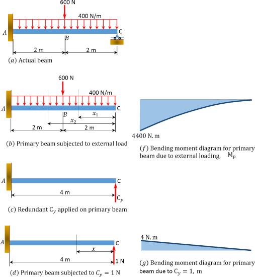
Determine the support reactions and draw the bending moment and the shearing force diagrams for the indeterminate beam shown in Figure 10.4. Use the method of consistent deformation. \(EI\) = constant.

\(Fig. 10.4\). Indeterminate beam.

Solution

Classification of structure. There are four unknown reactions in the beam: three unknown reactions at the fixed end \(A\) and one unknown reaction at the prop \(C\). Since there are three equations of equilibrium on a plane, it implies that the beam has one unknown reaction in excess of the equations of equilibrium on a plane. Thus, it is indeterminate to one degree.

Choice of primary structure. There may be more than one possible choice of primary structure. For the given propped cantilever beam, the reaction at \(C\) is selected as the redundant reaction. Thus, the primary structure is as shown in Figure 10.4b.

Compatibility equation. The number of compatibility equations will always match the number of the redundant reactions in a given structure. For the given cantilever beam, the number of compatibility equations is one and is written as follows:

\(\Delta_{C P}+C_{y} \delta_{C C}=0\)

The flexibility or compatibility coefficients \(\Delta_{C P}\) and \(\delta_{C C}\) are computed using the integration method.

The bending moment expressions for segments \(AB\) and \(BC\) of the primary beam subjected to an external loading is written as follows:

\(\begin{array}{l}
0<x_{1}<2 \\
M=-\frac{400 x^{2}}{2}=-200 x^{2} \\
2<x_{2}<4 \\
M=-\frac{400 x^{2}}{2}-600(x-2)=-200 x^{2}-600(x-2)
\end{array}\)

The bending moment in the primary beam subjected to \(C_{y}=1 \mathrm{~N}\) is written as follows:

\(\begin{array}{l}
M=x \\
\Delta_{1 P}=\int_{0}^{2} \frac{m M p d x}{E I}+\int_{2}^{4} \frac{\mathrm{m} M p d x}{E I} \\
\Delta_{1 P}=\int_{0}^{2} \frac{(x)\left(-200 x^{2}\right) d x}{E I}+\int_{2}^{4} \frac{(x)\left[-200 x^{2}-600(x-2)\right] d x}{E I} \\
=-\frac{16800}{E I} \\
\Delta \delta_{C 1}=\int_{0}^{4} \frac{\left(x^{2}\right) d x}{E I} \\
=\frac{21.33}{E I}
\end{array}\)

Putting the computed flexibility coefficients into the compatibility equation suggests the following:

\(C_{y}=-\frac{\Delta_{C P}}{\delta_{c 1}}=\frac{16800}{21.33}=787.63 \mathrm{~N}\)

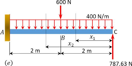
Shearing force and bending moment diagram. To determine the magnitudes of the shearing force and the bending moment and draw their diagrams, apply the obtained redundant to the primary beam, as shown in Figure 10.4e.

\(\begin{array}{l}
0<x_{1}<2 \\
V=-787.63+400 x \\
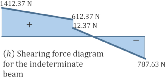
\text { When } x=0, V=-787.63 \mathrm{~N} \\
\text { When } x=2, V=12.37 \mathrm{~N} \\
M=787.63 x-\frac{400 x^{2}}{2} \\
\text { When } x=0, M=0 \\
\text { When } x=2, M=775.26 \mathrm{~N} . \mathrm{m}
\end{array}\)

\(\begin{array}{l}
2<x_{2}<4 \\
V=-787.63+400 x+600 \\
\text { When } x=2 \mathrm{~m}, V=612.37 \mathrm{~N} \\
\text { When } x=4 \mathrm{~m}, V=1412.37 \mathrm{~N} \\
M=787.63 x-\frac{400 x^{2}}{2}-600(x-2) \\
\text { When } x=2 \mathrm{~m}, M=775.26 \mathrm{~N} . \mathrm{m} \\
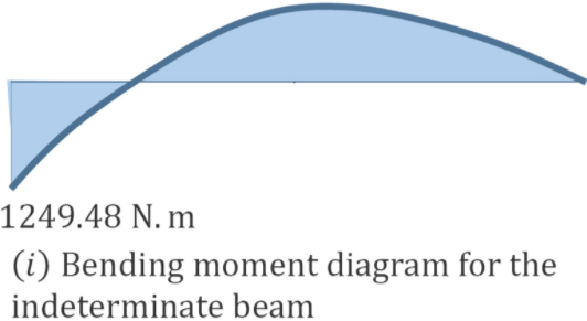
\text { When } x=4 \mathrm{~m}, M=-1249.48 \mathrm{~N} . \mathrm{m}
\end{array}\)

The shearing force and the bending moment diagrams are shown in Figure 10.4h and Figure 10.4i.

 

Computation of Flexibility Coefficients by Graph Multiplication Method

The computation of the flexibility coefficients for the compatibility equations by the method of integration can be very lengthy and cumbersome, especially for indeterminate structures with several unknown redundant forces. In such instances, obtaining the coefficients by the graph multiplication method is time-saving. The graph multiplication method is based on the premise that the integral \(\int \frac{M m}{E I} d x\) contains the product of two moment graphs \(M\) and \(m\). To derive the formula for the graph multiplication method, consider the two moment diagrams \(M^{\prime}\) and \(M\), as shown in Figure 10.5. The graph of \(M^{\prime}\) is linear, while that of \(M\) is of an arbitrary function.

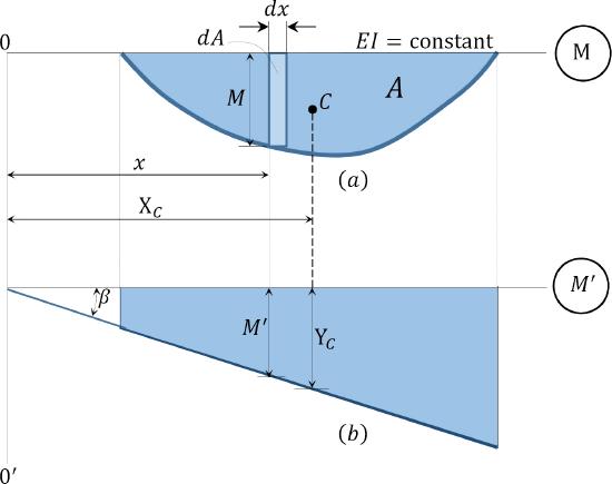
\(Fig. 10.5\). Moment diagrams.

Assuming the flexural rigidity \(EI\) is constant, the integral of the product of these two moment diagrams can be expressed as follows: \[\int \frac{M M^{\prime}}{E I} d x\]

The elementary area of the bending moment diagram at a distance \(x\) from the left end, as shown in Figure 10.5a, is written as follows: \[d A=M d x\]

Using trigonometry, the ordinate \(M^{\prime}\) of the linear graph \(M^{\prime}\) at a distance \(x\) from the origin, as shown in Figure 10.5b, can be expressed as follows: \[Y_{c}=x. \tan \beta\]

Substituting equation 2 and 3 into equation 1 suggests the following: \[\begin{aligned}
\int \frac{M m}{E I} d x &=\int d A . x . \tan \varphi \\
&=\tan \beta \int d A . x \\
&=x \tan \beta . A \\
&=A Y_{c} \\
\int \frac{M M}{E I} d x &=A Y_{c}
\end{aligned}\]

As suggested by equation 10.6, the integral of the product of two moment diagrams is equal to the product of the area of one of the moment diagrams (preferably the diagram with the arbitrary outline) and the ordinate in the second moment diagram with a straight outline, lying on a vertical line passing through the centroid of the first moment diagram.

Example 10.3

Determine the reactions at supports \(A\), \(C\), and \(D\) of the beam shown in Figure 10.6a. \(A\) is a fixed support, while \(C\) and \(D\) are roller supports. \(EI\) = constant.

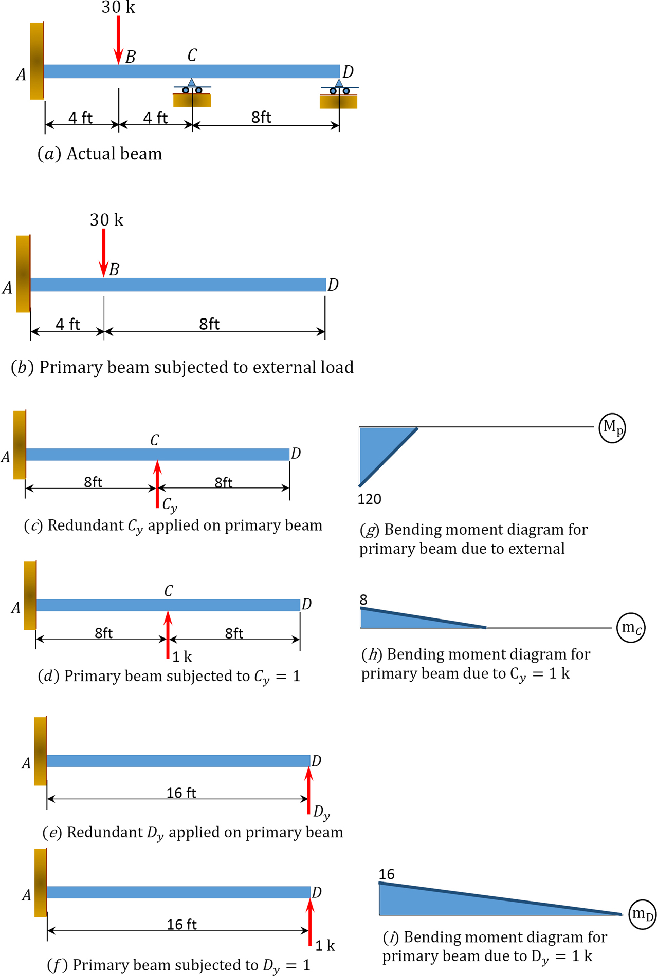
\(Fig. 10.6\). Beam.

Solution

Classification of structure. There are five unknown reactions in the beam. Thus, the degree of indeterminacy of the structure is two.

Choice of primary structure. The supports at \(C\) and \(D\) are chosen as the redundant reactions. Therefore, the primary structure is a cantilever beam subjected to the given concentrated load shown in Figure 10.6b. The primary structure subjected to the redundant unknowns are shown in Figure 10.6c, Figure 10.6d, Figure 10.6e, and Figure 10.6f.

Compatibility equation. There are two compatibility equations, as there are two redundant unknown reactions. The equations are as follows:

\(\begin{array}{l}
\Delta_{C P}+C_{y} \delta_{C C}+D_{y} \delta_{C D}=0 \\
\Delta_{D P}+C_{y} \delta_{D C}+D_{y} \delta_{D D}=0
\end{array}\)

The first alphabets of the subscript of the flexibility coefficients indicate the location of the deflection, while the second alphabets indicate the force causing the deflection. Using the graph multiplication method, the coefficients are computed as follows:

Using the graph multiplication method, the flexibility coefficients are computed as follows:

\(\begin{array}{l}
\Delta_{C P}=\left(-\frac{1}{2} \times 4 \times 120\right)(6.67)=-1600.8 \\
\Delta_{D P}=\left(-\frac{1}{2} \times 4 \times 120\right)(10.67)=-2560 \\
\delta_{C C}=\left(\frac{1}{2} \times 8 \times 8\right)(5.33)=170.56 \\
\delta_{C D}=\delta_{D C}=\left(\frac{1}{2} \times 8 \times 8\right)(13.33)=426.56 \\
\delta_{D D}=\left(\frac{1}{2} \times 16 \times 16\right)(10.67)=1365.76
\end{array}\)

Substituting the flexibility coefficients into the compatibility equation suggests the following two equations, with two unknowns:

\(\begin{array}{l}
-1600.8+170.56 C_{y}+426.56 D_{y}=0 \\
-2560+426.56 C_{y}+1365.76 D_{y}=0
\end{array}\)

Solving both equations simultaneously suggests the following:

\(C_{y}=21.46 \mathrm{k}\)

\(D_{y}=-4.83 \mathrm{k}\)

The determination of the reactions at support \(A\) is as follows:

\(\begin{array}{l}
+ \curvearrowleft \sum M_{A}=0:-(30)(4)-(4.83)(16)+(21.46)(8)+M_{A}=0 \\
M_{A}=25.6 \mathrm{k} . \mathrm{ft} \\
+\uparrow \sum F_{y} =0: A_{y}-30+21.46-4.83=0 \\
A_{y}=13.37 \mathrm{k} \\
+\rightarrow \sum F_{x}=0: A_{x}=0
\end{array}\)

Use of Beam-Deflection Tables for Computation of Flexibility Coefficients

This is the easiest method of computation of flexibility coefficients. It involves obtaining the constants from tabulated deflections based on the types of supports and loading configurations, as shown in Table 10.1 and Table 10.2.

\(Table 10.1\). Simply supported beam slopes and deflections.

Beam	Slope	Deflection	Elastic Curve
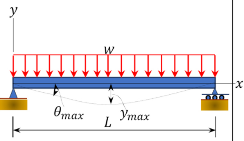	\(\begin{array}{l} \theta_{\max } \\ =\frac{-w L^{3}}{24 E I} \end{array}\)
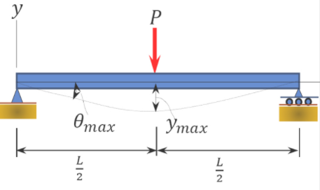	\(\theta_{\max }=\frac{-P L^{2}}{16 E I}\)	\(y_{\max }=\frac{-P L^{3}}{48 E I}\)	\(\begin{array}{c} 0 \leq x \leq \frac{L}{2} \\ y=\frac{-P x}{48 E I}\left(3 L^{2}-4 x^{2}\right) \end{array}\)
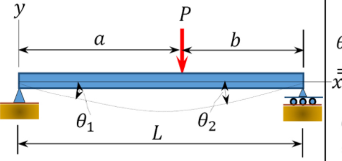	\(\begin{array}{l} \theta_{1} \\ =\frac{-P a b(L+b)}{6 E I L} \\ \theta_{2} \\ =\frac{P a b(L+a)}{6 E I L} \end{array}\)	\(\begin{array}{l} \text { At } x=a \\ y=\frac{-P b a}{6 E I}\left(L^{2}-b^{2}-a^{2}\right) \end{array}\)	\(\begin{array}{c} 0 \leq x \leq a \\ y=\frac{-P b x}{6 E I L}\left(L^{2}-b^{2}-x^{2}\right) \end{array}\)
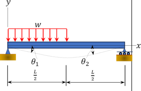	\(\begin{array}{l} \theta_{1}=\frac{-3 w L^{3}}{128 E I} \\ \theta_{2}=\frac{7 w L^{3}}{384 E I} \end{array}\)	\(\begin{aligned} \text { At } x=& \frac{L}{2} \\ & y=\frac{-5 w L^{4}}{768 E I} \\ & v_{\max } \text { is at } x \\ &=0.4598 L \\ V_{\max } &=-0.006563 \frac{w L^{4}}{E I} \end{aligned}\)	\(\begin{array}{c} 0 \leq x \leq \frac{L}{2} \\ y=\frac{-w x}{384 E I}\left(16 x^{3}-24 L x^{2}\right. \\ \left.+9 L^{3}\right) \\ \frac{L}{2} \leq x<L \\ y=\frac{-w L}{384 E I}\left(8 x^{3}-24 L x^{2}\right. \\ +17 L^{2} x \\ \left.-L^{3}\right) \end{array}\)
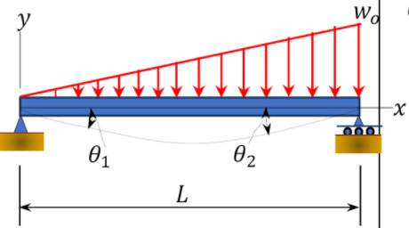	\(\begin{array}{c} \theta_{1}=\frac{-7 w_{O} L^{3}}{360 E I} \\ \theta_{2}=\frac{w_{0} L^{3}}{45 E I} \end{array}\)	\(\begin{aligned} &v_{\max } \text { is at } x=0.5193\\ &V_{\max }=-0.00652 \frac{w_{o} L^{4}}{E I} \end{aligned}\)	\(\begin{array}{r} y=\frac{-w_{0} x}{360 E I L}\left(3 x^{4}-10 L^{2} x^{2}\right. \\ \left.+7 L^{4}\right) \end{array}\)
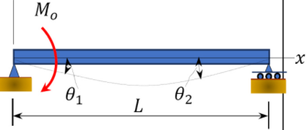	\(\begin{array}{c} \theta_{1}=\frac{-M_{0} L}{3 E I} \\ \theta_{2}=\frac{M_{o} L}{6 E I} \end{array}\)	\(y_{\max }=\frac{-M_{o} L^{2}}{\sqrt{243} E I}\)

\(Table 10.2\). Cantilevered beam slopes and deflections.

 

Beam	Slope	Deflection	Elastic Curve
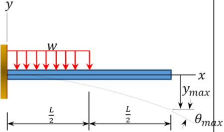	\(\theta_{\max }=\frac{-w L^{3}}{48 E I}\)		\(\begin{array}{c} 0 \leq x \leq \frac{L}{2} \\ y=\frac{-w x^{2}}{24 E I}\left(x^{2}-2 L x+\frac{3}{2} L^{2}\right) \\ \frac{L}{2} \leq x \leq L \\ y=\frac{-w L^{3}}{192 E I}\left(4 x-\frac{L}{2}\right) \end{array}\)
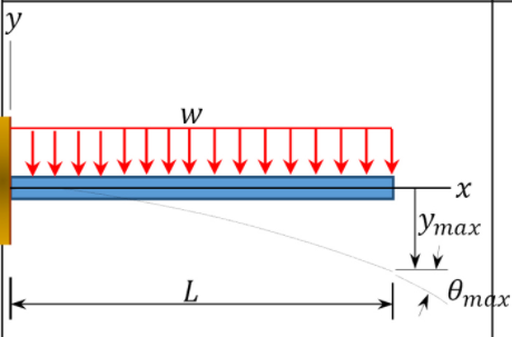	\(\theta_{\max }=\frac{-w L^{3}}{6 E I}\)	\(y_{\max }=\frac{-w L^{4}}{8 E I}\)
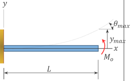	\(\theta_{\max }=\frac{M_{o} L}{E I}\)	\(y_{\max }=\frac{M_{o} L^{2}}{2 E I}\)	\(y=\frac{M_{0} x^{2}}{2 E I}\)
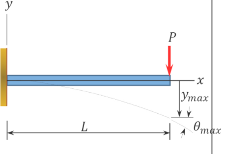	\(\theta_{\max }=\frac{-P L^{2}}{2 E I}\)	\(y_{\max }=\frac{-P L^{3}}{3 E I}\)	\(y=\frac{-P x^{2}}{6 E I}(3 L-x)\)
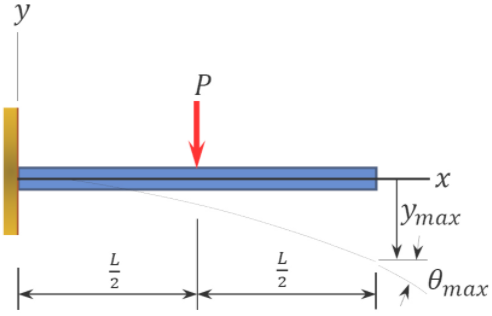	\(\theta_{\max }=\frac{-P L^{2}}{8 E I}\)		\(\begin{array}{r} 0 \leq x \leq \frac{L}{2} \\ y=\frac{-P x^{2}}{6 E I}\left(\frac{3}{2} L-x\right) \\ \frac{L}{2} \leq x \leq L \\ y=\frac{-P L^{2}}{24 E I}\left(3 x-\frac{L}{2}\right) \end{array}\)

Example 10.4

Draw the bending moment and the shearing force for the indeterminate beam shown in Figure 10.7a. \(EI\) = constant.

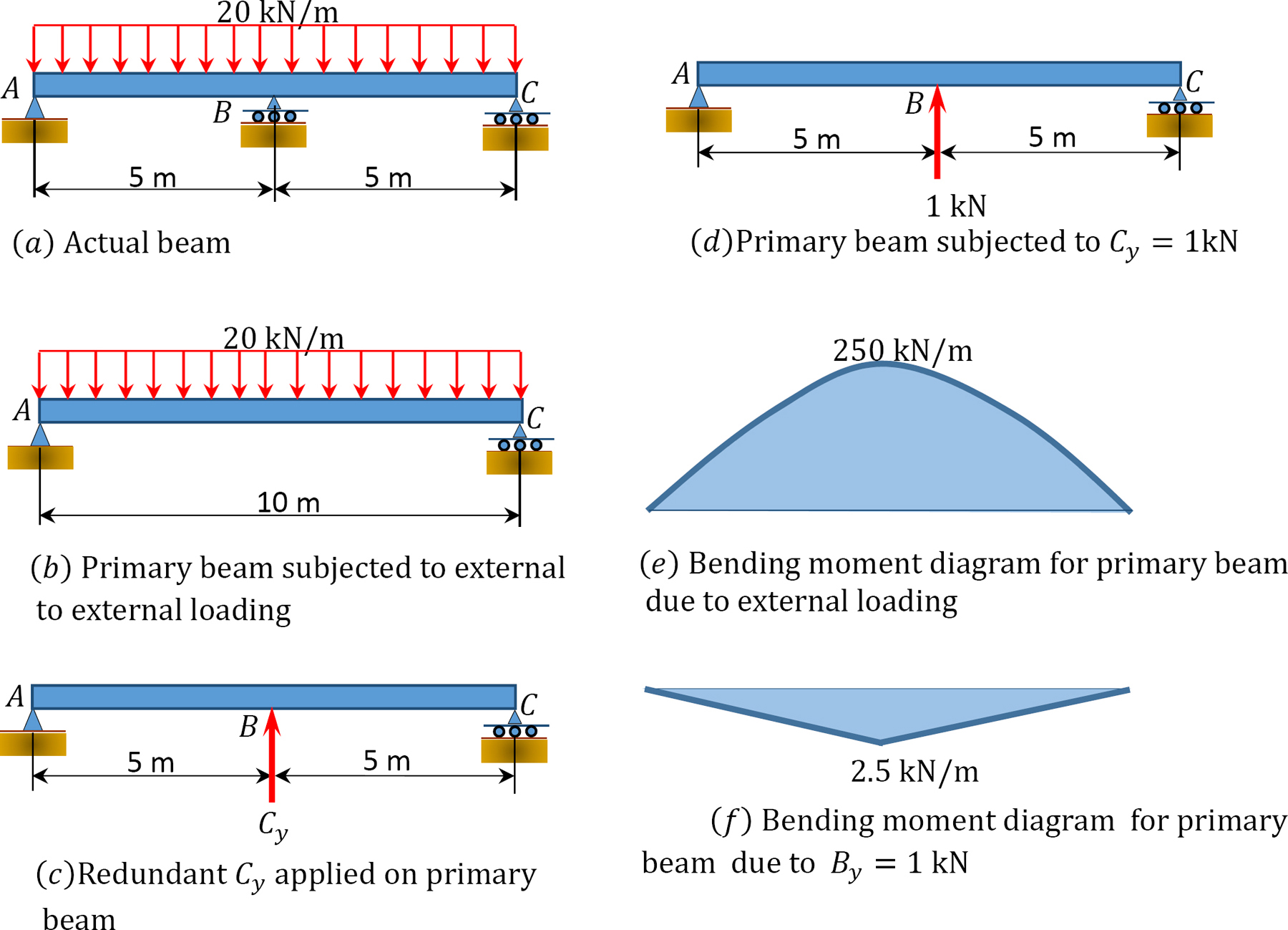
\(Fig. 10.7\). Indeterminate beam.

Solution

Classification of structure. There are four unknown reactions in the beam. Thus, the beam is indeterminate to one degree.

Choice of primary structure. The reaction at \(B\) is chosen as the redundant reaction. Thus, the primary structure is a simply supported beam, as shown in Figure 10.7b. Shown in Figure 10.7c and Figure 10.7d are the primary structures loaded with the redundant reactions.

Compatibility equation. The compatibility equation for the beam is written as follows:

\(\Delta_{B P}+B_{y} \delta_{B B}=0\)

To compute the flexibility coefficients \(\Delta_{B P}\) and \(\delta_{B B}\), use the beam-deflection formulas in Table 10.1.

\(\Delta_{B P}=-\frac{5 \omega L^{4}}{384 E I}=-\frac{5(20)(10)^{4}}{384 E I}=-\frac{2604.17}{E I}\)

\(\delta_{B B}=\frac{P L^{3}}{48 E I}=\frac{(10)^{3}}{48 E I}=\frac{20.83}{E I}\)

Putting the computed flexibility coefficients into the compatibility equation suggests the following:

\(B_{y}=\frac{\Delta_{B P}}{\delta_{B B}}=\frac{264.17}{20.83}=125 \mathrm{kN}\)

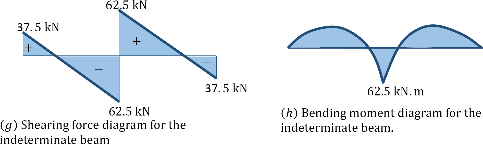
Shearing force and bending moment diagrams. Once the magnitudes of the redundant reactions are known, the beam becomes determinate and the bending moment and shearing force diagrams are drawn, as shown in Figure 10.7g and Figure 10.7h.

Example 10.5

To obtain the flexibility coefficients, use the beam-deflection tables to determine the support reactions of the beams in examples 10.1 and 10.2.

Solution

Classification of structure. The degree of indeterminacy of the beam in examples 10.1 and 10.2 is 2.

Flexibility coefficients. Using the information in Table 10.2, determine the flexibility coefficients for example 10.1, as follows:

\(\begin{array}{l}
\Delta_{B P}=-\frac{P L^{4}}{8 E I}=-\frac{q L^{4}}{8 E I} \\
\delta_{B B}=\frac{P L^{3}}{3 E I}=\frac{q L^{3}}{3 E I} \\
B_{y}=-\frac{\Delta_{B P}}{\delta_{B B}}=-\left(-\frac{q L^{4}}{8 E I}\right)\left(\frac{3 E I}{L^{3}}\right)=\frac{3 q L}{8}
\end{array}\)

Using the beam-deflection formulas, obtain the following flexibility coefficients for the beam in example 10.2, as follows:

\(\begin{array}{l}
\Delta_{C P}=\frac{-w L^{4}}{8 E I}+\frac{-5 P L^{3}}{48 E I}=\frac{-400(4)^{4}}{8 E I}+\frac{-5(600)(4)^{3}}{48 E I}=-\frac{16800}{E I} \\
\delta_{C C}=\frac{P L^{3}}{3 E I}=\frac{(1)(4)^{3}}{3 E I}=\frac{21.33}{E I}
\end{array}\)

Putting the computed flexibility coefficients into the compatibility equation suggests the following answer:

\(C_{y}=-\frac{\Delta_{C P}}{\delta_{C C}}=\frac{16800}{21.33}=787.63 \mathrm{~N}\)

Example 10.6

Using the method of consistent deformation, draw the shearing force and the bending moment diagrams of the frame shown in Figure 10.8a. \(EI\) = constant.

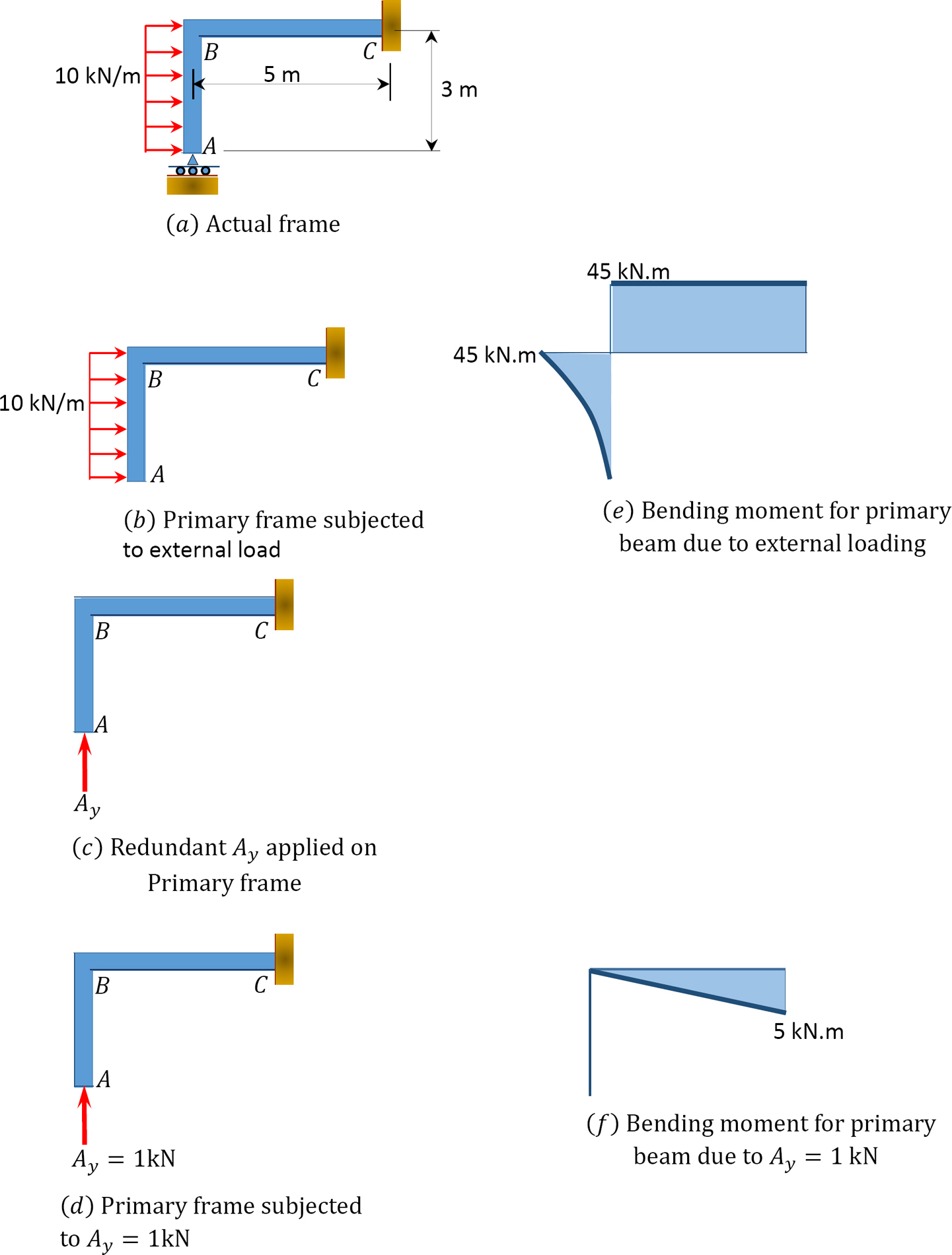
\(Fig. 10.8\). Frame.

Solution

Classification of structure. There are four unknown reactions in the frame: one unknown reaction at the free end \(A\) and three unknown reactions at the fixed end \(C\). Thus, the degree of indeterminacy of the structure is one.

Choice of primary structure. Selecting the reaction at support \(A\) as the redundant unknown force suggests that the primary structure is as shown in Figure 10.8b. The primary structure loaded with the redundant force is shown Figure 10.8c and Figure 10.8d.

Compatibility equation. The compatibility equation for the indeterminate frame is as follows:

\(\Delta_{A P}+A_{v} \delta_{A A}=0\)

The flexibility or compatibility coefficients \(\Delta_{A P}\) and \(\delta_{A A}\) are computed by graph multiplication method, as follows:

\(\begin{array}{c}
\Delta_{B P}=-\frac{1}{2}(5 \times 5)(45)=-562.5 \\
\delta_{A A}=\frac{1}{2}(5 \times 5)\left(\frac{10}{3}\right)=41.67
\end{array}\)

Substituting the flexibility coefficients into the compatibility equation and solving it to obtain the redundant reaction suggests the following:

\(\begin{array}{l}
-562.5+41.67 A_{Y}=0 \\
A_{Y}=13.5 \mathrm{kN}
\end{array}\)

Determining the reactions at \(C\).

\begin{aligned}
\sum M_{c}=0:-(13.5)(5)+(10 \times 3)(1.5)+M_{c}=0\\
M_{c}=22.5 .6 \text { kN. m}\\
\sum F_{y}=0:-C_{y}+13.5=0 \\
C_{y}=13.5 \mathrm{kN} \\
\sum F_{x}=0:-C_{x}+(10 \times 3)=0 \\
\mathrm{C}_{x}=30 \mathrm{kN}
\end{aligned}

Example 10.7

Using the method of consistent deformation, determine the support reactions of the truss shown in Figure 10.9a. \(EI\) = constant.

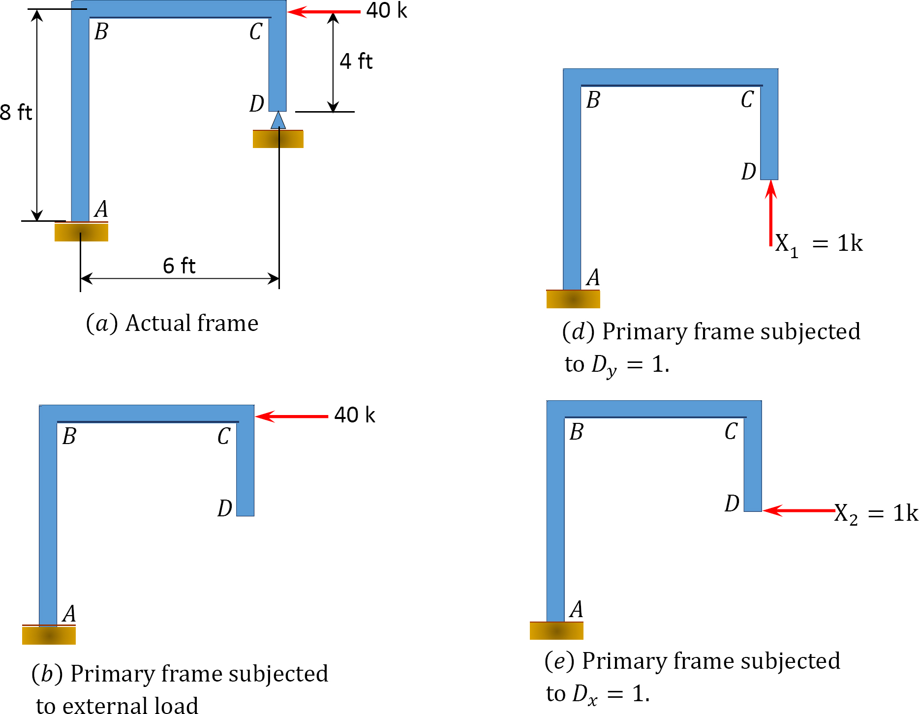
\(Fig. 10.9\). Truss.

Solution

Classification of structure. There are five unknown reactions in the beam. Thus, the degree of indeterminacy of the structure is two.

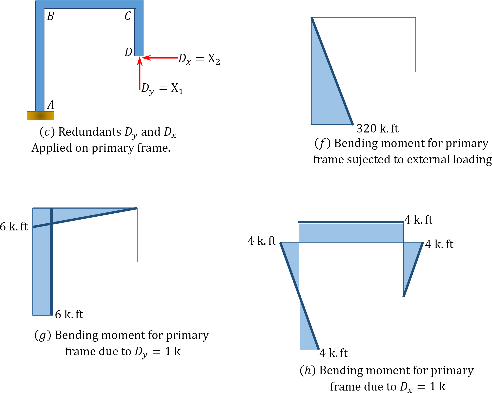
Choice of primary structure. The two reactions of the pin support at \(D\) are chosen as the redundant reactions, therefore the primary structure is a cantilever beam subjected to a horizontal load at \(C\), as shown in Figure 10.9b. The primary structure loaded with the redundant unknowns is shown in Figure 10.9d and Figure 10.9e.

Compatibility equation. The number of compatibility equations is two, since there are two redundant unknowns. The equations are written as follows:

\(\begin{array}{l}
\Delta_{1 P}+X_{1} \delta_{11}+X_{2} \delta_{12}=0 \\
\Delta_{2 P}+X_{1} \delta_{21}+X_{2} \delta_{22}=0
\end{array}\)

The first number of the subscript in the flexibility coefficients indicates the direction of the deflection, while the second number or letter indicates the force causing the deflection. The coefficients are computed using the graph multiplication method, as follows:

\(\begin{array}{l}
\Delta_{1 P}=\frac{1}{E I}\left(\frac{1}{2} \times 8 \times 320\right)(6)=\frac{7680}{E I} \\
\Delta_{2 P}=\frac{1}{E I}\left(-\frac{1}{2} \times 4 \times 4\right)(53.33)+\left(\frac{1}{2} \times 4 \times 4\right)(266.8)=\frac{1707.76}{E I} \\
\delta_{11}=\frac{1}{E I}\left(\frac{1}{2} \times 6 \times 6\right)(4)+(6 \times 8)(6)=\frac{360}{E I} \\
\delta_{12}=\delta_{21}=\frac{1}{E I}\left(-\frac{1}{2} \times 4 \times 4\right)(6)+\left(\frac{1}{2} \times 4 \times 4\right)(6)-\left(\frac{1}{2} \times 6 \times 6\right)(4)=-\frac{72}{E I} \\
\delta_{22}=\frac{1}{E I}(3)\left(\frac{1}{2} \times 4 \times 4\right)(2.67)+(4 \times 6)(4)=\frac{160.08}{E I}
\end{array}\)

Substituting the flexibility coefficients into the compatibility equation suggests the following two equations with two unknowns:

\(\begin{array}{l}
7680+360 X_{1}-72 X_{2}=0 \\
1707.76-72 X_{1}+160.08 X_{2}=0
\end{array}\)

Solving both equations simultaneously suggests the following:

\(\begin{array}{l}
X_{1}=D_{y}=25.79 \mathrm{k} \\
X_{2}=D_{X}=22.27 \mathrm{k}
\end{array}\)

Determination of the reactions at support \(A\).

\(\begin{array}{c}
\sum M_{A}=0:(25.79)(6)+(22.27)(16)+(21.46)(4)+M_{A}=0 \\
M_{A}=25.6 \mathrm{k} . \mathrm{ft} \\
\qquad \sum F_{y}=0: A_{y}-30+21.46-4.83=0 \\
A_{y}=13.37 \mathrm{k}
\end{array}\)