10.4: Analysis of Indeterminate Trusses

The procedure for the analysis of indeterminate trusses is similar to that followed in the analysis of beams. For trusses with external redundant restraints, the procedure entails determining the degree of indeterminacy of the structure, selecting the redundant reactions, writing the compatibility equations, determining the deflection due to the applied load and the one due to a unit redundant reaction force applied to the primary structure, and solving the compatibility equation(s) to determine the redundant reactions. For trusses with internal redundant members, the procedure involves selecting the redundant members, cutting the redundant members and depicting each of them as a pair of forces in the primary structure, and then applying the condition of compatibility to determine the axial forces in the redundant members. Consider the truss below for an example. This truss is indeterminate to the first degree. Members \(AC\) and \(BD\) of the truss are two separate overlapping members. Either of these members can be considered redundant, since the primary structure obtained after the removal of either of them will remain stable. Selecting \(BD\) as the redundant member, cutting through it and applying a pair of forces on the cut surface, and then indicating that the displacement of the truss at the cut surface is zero suggests the following compatibility expression: \[\Delta_{B D}+F_{B D} \delta_{B D}=0\]

where\(\begin{array}{c}
M_{C B}=\frac{2 \mathrm{EI}}{L}\left(\theta_{B}+2 \theta_{C}-3 \psi\right)+F E M_{C B} \\
2 \mathrm{EK} \theta_{B}+46.67
\end{array}\)

\(\Delta_{B D}\) = the relative displacement of the cut surface due to the applied load.

\(\delta_{B D}\) = the relative displacement of the cut surface due to an applied unit redundant load on the cut surface.

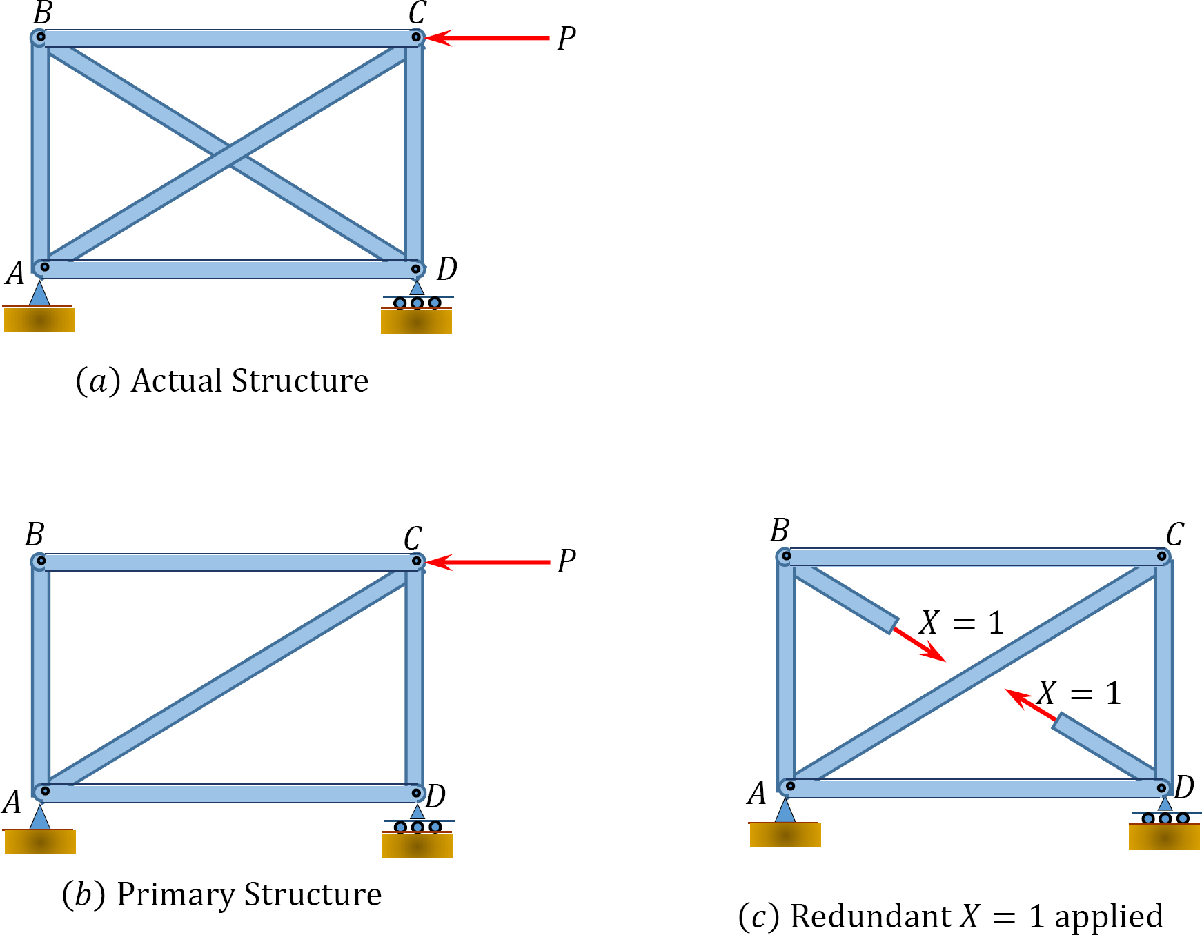
\(Fig. 10.10\)

The flexibility coefficients for the compatibility equation for the indeterminate truss analysis is computed as follows: \[\begin{array}{l}
\Delta_{X P}=\sum \frac{F f L}{A E} \\
\delta_{X X}=\sum \frac{f^{2} L}{A E}
\end{array}\]

where

\(\Delta_{X P}\) = the displacement at a joint \(X\) or member of the primary truss due to applied external load.

\(\delta_{X 1}\) = the displacement at joint X or member of the primary truss due to the unit redundant force.

\(F\) = axial force in the truss members due to the applied external load that causes the displacement \(\Delta\).

\(f\) = axial forces in truss members due to the applied unit redundant load that causes the displacement \(\delta\).

\(L\) = length of member.

\(A\) = cross sectional area of a member.

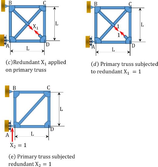
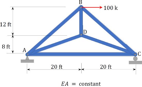
Example 10.8

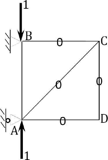
Using the method of consistent deformation, determine the axial force in all the members of the truss shown in Figure 10.11a. \(EA\) = constant. .

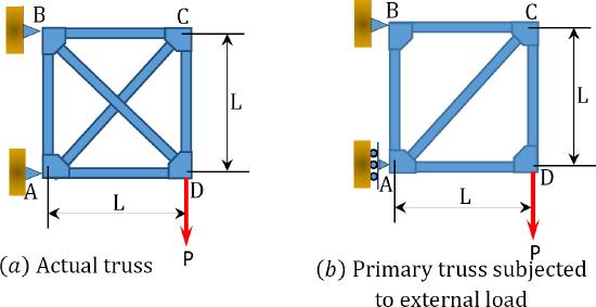
\(Fig. 10.11\). Truss.

Solution

Determining support reactions in the primary structure.

\(\begin{array}{l}
+ \curvearrowleft \sum M_{B}=0 \\
-P L+A_{x} L=0 \\
A_{x}=P
\end{array}\)

\(\begin{array}{l}
+\rightarrow \sum F_{x}=0 \\
-P+B_{x}=0 \\
B_{x}=P
\end{array}\)

\(\begin{array}{l}
+\uparrow \sum F_{y}=0 \\
-P-B_{y}=0 \\
B_{y}=P
\end{array}\)

Compatibility Equation.

\(\begin{array}{l}
\Delta_{1} p+\mathrm{X}_{1} \delta_{11}+\mathrm{X}_{2} \delta_{12}=0 \\
\Delta_{2} p+\mathrm{X}_{1} \delta_{21}+\mathrm{X}_{2} \delta_{22}=0
\end{array}\)

Determining forces in members due to applied external load.

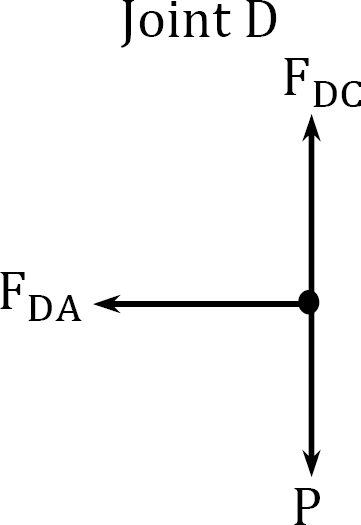
Joint \(D\).

\(\begin{array}{l}
+\uparrow \sum F_{y}=0: F_{D C}-P=0 \\
F_{D C}=P \\
+\rightarrow \sum F_{x}=0: F_{D A}=0
\end{array}\)

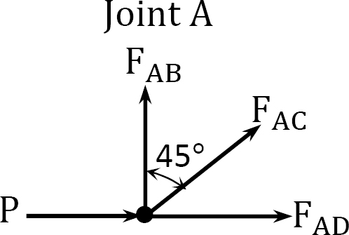
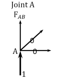
Joint \(A\).

\(\begin{array}{l}
\rightarrow \sum F_{x}=0: F_{A C} \cos 45^{\circ}+F_{A D}+P=0 \\
F_{A C}=-\frac{P}{\cos 45^{\circ}}=-1.414 P \\
+\uparrow \sum F_{y}=0: F_{A B}+F_{A C} \cos 45^{\circ}=0 \\
F_{A B}=-(-1.414 P) \cos 45^{\circ}=P
\end{array}\)

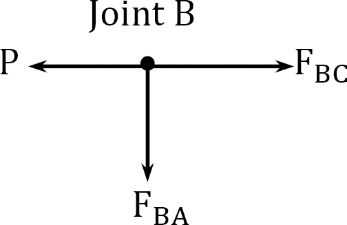
Joint \(B\).

\(+\rightarrow \sum F_{x}=0:-P+F_{B C}=0 ; F_{B C}=P\)

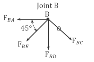
Determining forces in members due to redundant \(F_{B D} = 1\).

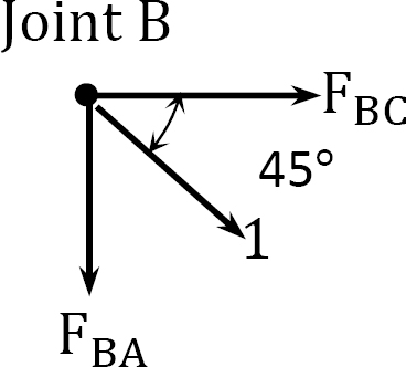
Joint \(B\).

\(\begin{array}{l}
+\rightarrow \sum F_{x}=0: 1 \cos 45^{\circ}+F_{B C}=0 ; F_{B C}=-\cos 45^{\circ}=-0.7071 \\
+\uparrow \sum F_{y}=0:-1 \cos 45^{\circ}-F_{B A}=0 ; F_{B A}=-0.7071
\end{array}\)

Joint \(D\).

 

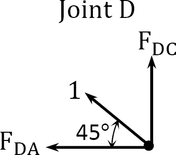
\(+\uparrow \sum F_{y}=0: 1 \cos 45^{\circ}+F_{D C}=0 ; F_{D C}=-0.7071\)

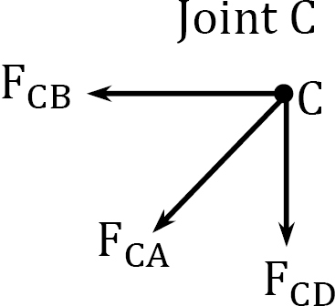
Joint \(C\).

\(+\uparrow \sum F_{y}=0:-F_{C A} \cos 45^{\circ}-F_{C D}=0 ; F_{C A}=1\)

Determining forces in members due to redundant \(A_{y}=1\).

Joint \(A\).

\(\begin{array}{r}
+\uparrow \sum F_{y}=0: 1+F_{A B}=0 \\
F_{A B}=-1
\end{array}\)

The determination of the member-axial forces can be conveniently performed in a tabular form, as shown in Table 10.3.

\(Table 10.3\).

Member	Length	N	\(n_{BD}\)	\(n_A\)	\(n_{BD}^2L\)	\(n_{A}^2L\)	\(n_{BD}n_AL\)	\(Nn_{BD}L\)	\(Nn_AL\)
AB	L	P	-0.7071	-1	0.5L	L	0.7071L	-0.7071PL	-PL
AC	1.414L	-1.414P	1	0	1.414L	0	0	-2PL	0
AD	L	0	-0.7071	0	0.5L	0	0	0	0
BC	L	P	-0.7071	0	0.5L	0	0	-0.7071PL	0
BD	1.414L	0	1	0	1.414L	0	0	0	0
CD	L	P	-0.7071	0	0.5L	0	0	-0.7071PL	0
Total					4.828L	L	0.7071L	-4.12PL	-PL

\(\begin{array}{l}
\Delta_{1 P}=-\frac{4.12 P L}{E A} \\
\Delta_{2 P}=-\frac{P L}{E A} \\
\delta_{11}=\frac{4.828 L}{E A} \\
\delta_{12}=\delta_{12}=\frac{0.7071 L}{E A} \\
\delta_{22}=\frac{L}{E A}
\end{array}\)

Substituting the flexibility coefficient into the compatibility equations and solving the simultaneous equations suggests the following:

\(\begin{array}{c}
-4.12 P+4.828 X_{1}+0.7071 X_{2}=0 \\
-P+0.7071 X_{1}+X_{2}=0
\end{array}\)

\(\begin{array}{l}
X_{1}=F_{B D}=0.79 \mathrm{P} \\
X_{2}=A_{y}=0.44 \mathrm{P}
\end{array}\)

The axial forces in members are as follows:

\(F_{AB}=P+(0.79P)(-0.7071)+(0.44P)(-1)=0.0014P\)

\(F_{AC}=-1.414P+(1)(0.79P)=-0.624P\)

\(F_{AD}=(-0.7071)(0.79P)=-0.559P\)

\(F_{BC}=P+(-0.7071)(0.79P)=0.441P\)

\(F_{BD}=0.79P\)

\(F_{CD}=P+(-0.7071)(0.79P)=0.441P\)

Example 10.9

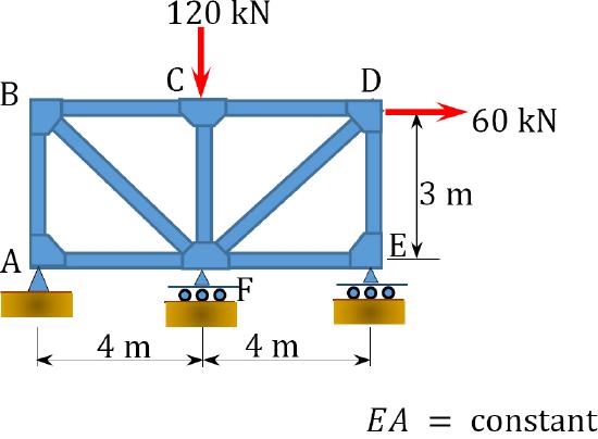
Using the method of consistent deformation, determine the axial force in member \(AD\) of the truss shown in Figure 10.12a. \(EA\) = constant.

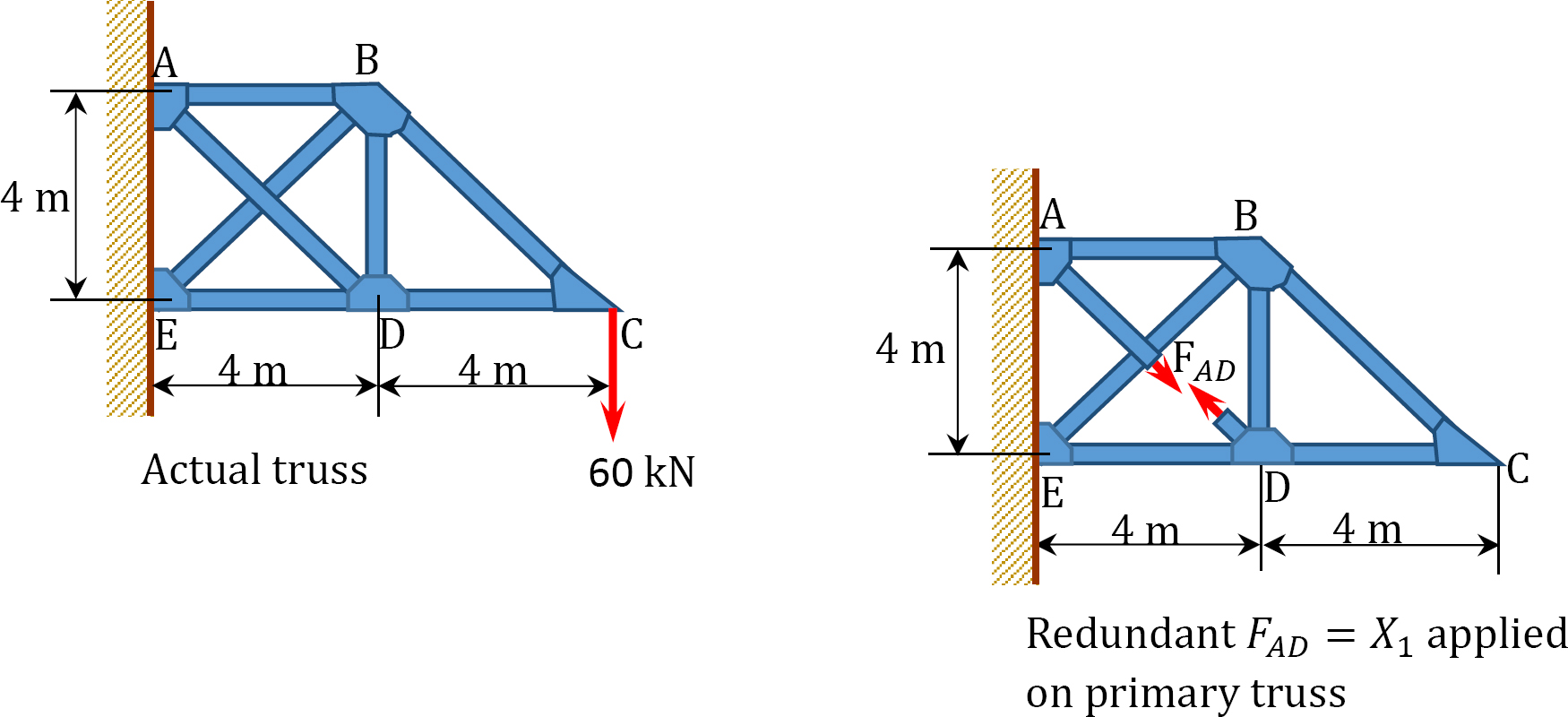
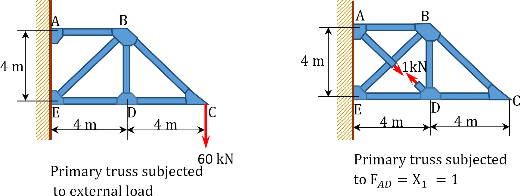
\(Fig. 10.12\). Truss.

Solution

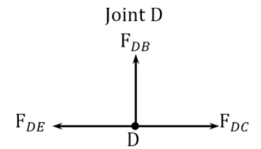
Determination of axial forces in members due to applied external loads.

\(\begin{aligned}
+\uparrow \sum F_{y}=0: F_{B C} \sin 45^{\circ}-60=0 & \\
\quad F_{B C}=84.85 \mathrm{kN} \\
+\rightarrow \sum F_{x}=0:-F_{C D}-F_{B C} \cos 45^{\circ}=0 \\
F_{C D}=-84.85 \cos 45^{\circ}=-60 \mathrm{kN}
\end{aligned}\)

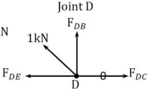
\(\begin{array}{l}
+\uparrow \sum F_{y}=0: F_{D B}=0 \\
\rightarrow \sum F_{x}=0: F_{D E}=F_{D C}=-60 \mathrm{kN}
\end{array}\)

Determining forces in members due to redundant \(F_{A D}=1\).

\(\begin{array}{l}
+\uparrow \sum F_{y}=0: \cos 45^{\circ}+F_{D B}=0 \\
F_{D B}=-\cos 45^{\circ} \mathrm{kN}=-0.7071 \mathrm{kN} \\
+\rightarrow \sum F_{x}=0:-F_{D E}-\cos 45^{\circ}=0 \\
F_{D E}=-0.7071 \mathrm{kN}
\end{array}\)

\(\begin{array}{l}
+\uparrow \sum F_{y}=0:-F_{B E} \cos 45^{\circ}-F_{B D}=0 \\
F_{B E}=-\frac{F_{B D}}{\operatorname{Cos} 45^{\circ}}=\frac{0.7071}{0.7071}=1 \mathrm{kN} \\
+\rightarrow \sum F_{x}=0:-F_{B A}-F_{B E} \cos 45^{\circ}=0 \\
F_{B A}=-0.7071 \mathrm{kN}
\end{array}\)

The determination of the member-axial forces can be conveniently performed in a tabular form, as shown in Table 10.4.

\(Table 10.4\).

Member	Length (m)	N (kN)	\(n_{AD}\)(kN)	N\(n_{AD}\)L	\(n^2_{AD}\)L
AB	4	120	-0.7071	-339.41	2.0
AD	5.66	0	1	0	5.66
BE	5.66	-84.85	1	-480.25	5.66
BD	4	0	-0.7071	0	2
BC	5.66	84.85	0	0	0
CD	4	-60	0	0	0
DE	4	-60	-0.7071	169.7	2
				-649.96	17.32

Compatibility equation.

\(\begin{array}{l}
\Delta_{1 P}+X_{1} \delta_{11}=0 \\
F_{A D}=X_{1}=-\frac{\Delta_{1 p}}{\delta_{11}}=\frac{649.96}{17.32}=37.53 \mathrm{kN}
\end{array}\)

Chapter Summary

Force method: The force method or the method of consistent deformation is based on the equilibrium of forces and compatibility of structures. The method entails first selecting the unknown redundants for the structure and then removing the redundant reactions or members to obtain the primary structure.

Compatibility equations: The compatibility equations are formulated and used together with the equations of equilibrium to determine the unknown redundants. The number of the compatibility equations must match the number of the unknown redundants. Once the unknown redundants are determined, the structure becomes determinate. Methods of computation of compatibility or flexibility coefficients, such as the method of integration, the graph multiplication method, and the use of deflection tables, are solved in the chapter.

Mohr integral for computation of flexibility coefficients for beams and frames:

\(\begin{array}{l}
\Delta_{B P}=\int \frac{M m}{E I} d x \\
\delta_{B B}=\int \frac{m^{2}}{E I} d x \\
\theta_{A P}=\int \frac{M m_{\theta}}{E I} d x \\
\alpha_{A A}=\int \frac{m_{\theta}^{2}}{E I} d x
\end{array}\)

Maxwell-Betti law of reciprocal deflections: The Maxwell-Betti law helps reduce the computational efforts required to obtain the flexibility coefficients for the compatibility equations. This law states that the linear displacement at point \(A\) due to a unit load applied at \(B\) is equal in magnitude to the linear displacement at point \(B\) due to a unit load applied at \(A\) for a stable elastic structure. This law is expressed as follows:

\(\delta_{A B}=\delta_{B A}\)

Practice Problems

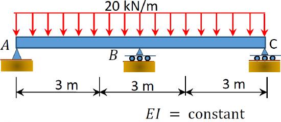
10.1 Using the method of consistent deformation, compute the support reactions and draw the shear force and the bending moment diagrams for the beams shown in Figures P10.1 through P10.4. Choose the reaction at the interior support \(B\) as the unknown redundant.

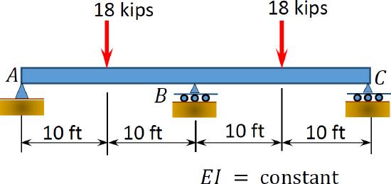
\(Fig. P10.1\). Beam.

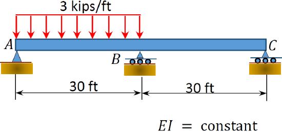
\(Fig. P10.2\). Beam.

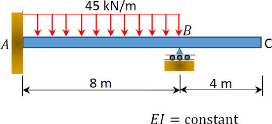
\(Fig. P10.3\). Beam.

\(Fig. P10.4\). Beam.

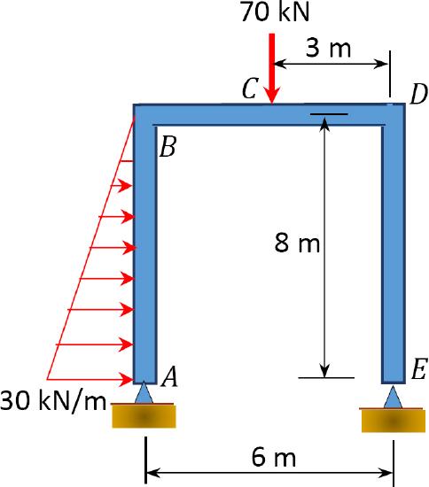
10.2 Using the method of consistent deformation, compute the support reactions and draw the shear force and the bending moment diagrams for the frames shown in Figures P10.5 through P10.8. Choose the reaction(s) at any of the supports as the unknown redundant(s). \(EI\) = constant.

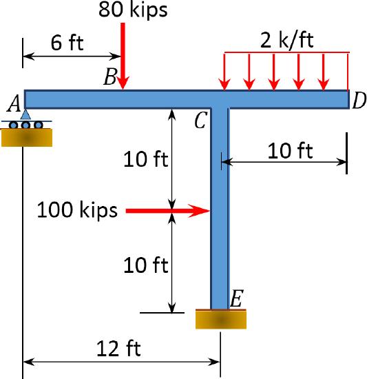
\(Fig. P10.5\). Frame.

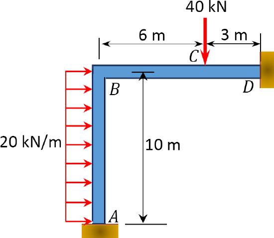
\(Fig. P10.6\). Frame.

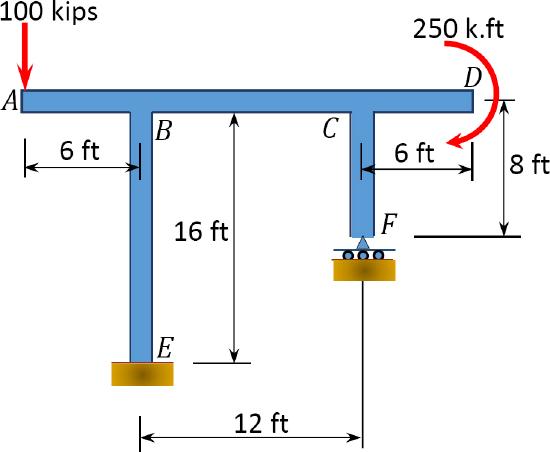
\(Fig. P10.7\). Frame.

\(Fig. P10.8\). Frame.

10.3 Using the method of consistent deformations, determine the reactions and the axial forces in the members of the trusses shown in Figures P10.9 through P10.13.

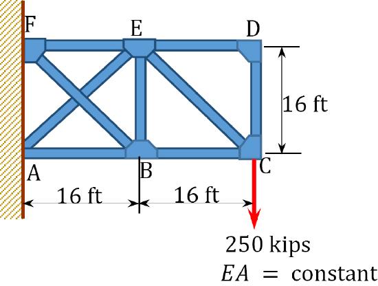
\(Fig. P10.9\). Truss.

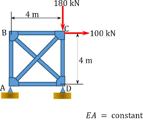
\(Fig. P10.10\). Truss.

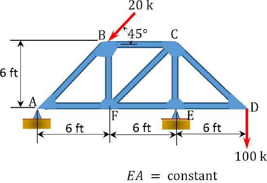
\(Fig. P10.11\). Truss.

\(Fig. P10.12\). Truss.

\(Fig. 10.13\). Truss.