12.6: Analysis of Indeterminate Frames

 

Procedure for Analysis of Indeterminate Sway-Frames by the Moment Distribution Method

A. Non-sway stage analysis

•First assume the existence of an imaginary prop that prevents the frame from swaying.

•Compute the horizontal reactions at the supports of the frame and note the difference X. This is the force to prevent sway.

B. Sway stage analysis

•Assume arbitrary moments to act on the columns of the frame. The magnitude of these moments will vary from column to column in proportion to \(\frac{I}{L^{2}}\).

•Values are assumed for \(M_{2}\), and \(M_{1}\) is determined.

•The arbitrary moments are then distributed as for the non-sway condition

•Calculate the magnitude of the horizontal reactions at the supports for the sway condition. The summation of these reactions gives the arbitrary displacing force \(Y\).

•Determine the ratio \(\frac{X}{Y}\). This ratio is called the sway factor.

•Use the sway factor to multiply the distributed moments of the sway. This gives the corrected moment for the sway.

•The final moments for the frame are the summation of the moments obtained in the non-sway stage and the corrected moment for the sway stage.

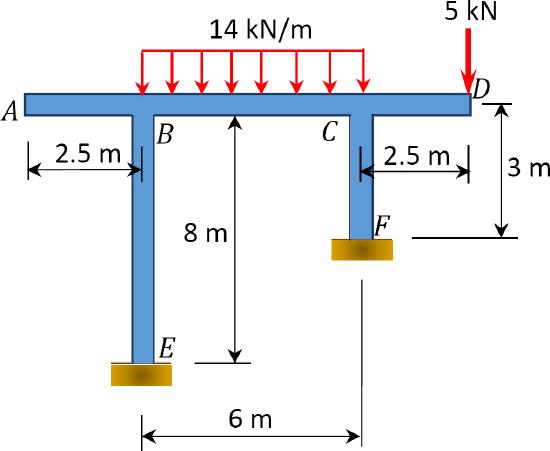
Example 12.3

Using the moment distribution method, determine the members’ end moments of the frame shown in Figure 12.8. \(EI =\) constant.

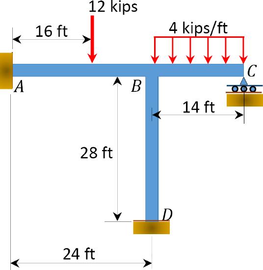
\(Fig. 12.8\). Frame.

Solution

Fixed end moment.

\(\begin{array}{l}
(F E M)_{A B}=-\frac{P a b^{2}}{L^{2}}=-\frac{12 \times 16 \times 8^{2}}{24^{2}}=-21.33 \mathrm{k.} \mathrm{ft} \\
(F E M)_{B A}=+\frac{P a^{2} b}{L^{2}}=\frac{12 \times 16^{2} \times 8}{24^{2}}=+42.67 \mathrm{k} . \mathrm{ft} \\
(F E M)_{B C}=-\frac{w L^{2}}{12}=-\frac{4 \times 14^{2}}{12}=-65.33 \mathrm{k.} \mathrm{ft} \\
(F E M)_{C B}=\frac{w L^{2}}{12}=+65.33 \mathrm{k} . \mathrm{ft}
\end{array}\)

Stiffness factor.

\(\begin{array}{l}
K_{A B}=K_{B A}=\frac{I_{A B}}{L_{A B}}=\frac{I}{24}=0.0417 \mathrm{I} \\
K_{B C}=K_{C B}=\frac{3}{4} \times \frac{I_{B C}}{L_{B C}}=\frac{3}{4} \times \frac{\mathrm{I}}{14}=0.0536 \mathrm{I} \\
K_{B D}=K_{D B}=\frac{I_{B D}}{L_{B D}}=\frac{I}{28}=0.0357 \mathrm{I}
\end{array}\)

Distribution factor.

\(\begin{array}{l}
(D F)_{A B}=\frac{K_{A B}}{\sum K}=\frac{K_{A B}}{K_{A B}+0}=\frac{0.0417 \mathrm{I}}{0.0417 \mathrm{I}+\infty}=0 \\
(D F)_{B A}=\frac{K_{B A}}{\sum K}=\frac{K_{B A}}{K_{B A}+K_{B C}+K_{B D}}=\frac{0.0417 \mathrm{I}}{0.0417 \mathrm{I}+0.0536 \mathrm{I}+0.0357 \mathrm{I}}=0.32 \\
(D F)_{B C}=\frac{K_{B C}}{\sum K}=\frac{K_{B C}}{K_{B A}+K_{B C}+K_{B D}}=\frac{0.0536 \mathrm{I}}{0.0417 \mathrm{I}+0.0536 \mathrm{I}+0.0357 \mathrm{I}}=0.41 \\
(D F)_{C B}=\frac{K_{C B}}{\sum K}=\frac{K_{C B}}{K_{C B}+0}=\frac{0.0536 \mathrm{I}}{0.0536 \mathrm{I}+0}=1 \\
(D F)_{B D}=\frac{K_{B D}}{\sum K}=\frac{K_{B D}}{K_{B A}+K_{B C}+K_{B D}}=\frac{0.0357 \mathrm{I}}{0.0417 \mathrm{I}+0.0536 \mathrm{I}+0.0357 \mathrm{I}}=0.27 \\
(D F)_{D B}=\frac{K_{D B}}{\sum K}=\frac{0.0357 \mathrm{I}}{0.0357 \mathrm{I}+\infty}=0
\end{array}\)

\(Table 12.3\). Distribution table.
 

Joint	A	B			C	D
Member	AB	BA	BC	BD	CB	DB
DF	0	0.32	0.41	0.27	1	0
FEM Dist. 1	-21.33	+42.67 +7.25	-65.33 +9.29	0 +6.12	+65.33 -65.33
CO Dist. 2	+3.625	+10.453	-32.665 +13.393	+8.82	+4.645 -4.645	+3.06
	+5.23					+4.41
Total	-12.48	+60.37	-75.31	+14.94	0.0	+7.47

Final member end moments.

Substituting the obtained values of \(E K \theta_{B}\), \(E K \theta_{C}\), and \(E K \Delta\) into the member end moment equations suggests the following:

\(\begin{array}{l}
M_{A B}=-12.48 \mathrm{k} . \mathrm{ft} \\
M_{B A}=+60.37 \mathrm{k} . \mathrm{ft} \\
M_{B C}=-75.31 \mathrm{k} . \mathrm{ft} \\
M_{B D}=+14.94 \mathrm{k} . \mathrm{ft} \\
M_{C B}=0 \\
M_{D B}=+7.47 \mathrm{k} . \mathrm{ft}
\end{array}\)

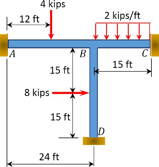
Example 12.4

Using the moment distribution method, determine the end moments at the supports of the frame shown in Figure 12.9. \(EI =\) constant.

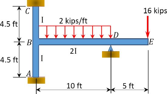
\(Fig. 12.9\). Frame.

Solution

Fixed end moment.

\(\begin{array}{l}
(F E M)_{A B}=(F E M)_{B A}=(F E M)_{B C}=(F E M)_{C B}=0 \\
(F E M)_{B D}=-\frac{w L^{2}}{12}=-\frac{2 \times 10^{2}}{12}=-16.67 \mathrm{k} . \mathrm{ft} \\
(F E M)_{D B}=\frac{w \mathrm{~L}^{2}}{12}=+16.67 \mathrm{k} . \mathrm{ft}
\end{array}\)

Stiffness factor.

\(\begin{array}{l}
K_{A B}=K_{B A}=\frac{I_{A B}}{L_{A B}}=\frac{\mathrm{I}}{4.5}=0.222 \mathrm{I} \\
K_{B C}=K_{C B}=\frac{I_{B C}}{L_{B C}}=\frac{\mathrm{I}}{4.5}=0.222 \mathrm{I} \\
K_{B D}=K_{D B}=\frac{3}{4} \times \frac{I_{B D}}{L_{B D}}=\frac{3}{4} \times \frac{2 \mathrm{I}}{10}=0.15 \mathrm{I}
\end{array}\)

Distribution factor.

\(\begin{array}{l}
(D F)_{A B}=0 \\
(D F)_{B A}=\frac{K_{B A}}{\sum K}=\frac{K_{B A}}{K_{B A}+K_{B C}+K_{B D}}=\frac{0.222 \mathrm{I}}{0.222 \mathrm{I}+0.222 \mathrm{I}+0.15 \mathrm{l}}=0.37 \\
(D F)_{B C}=\frac{K_{B C}}{\sum K}=\frac{K_{B A}}{K_{B A}+K_{B C}+K_{B D}}=\frac{0.222 \mathrm{I}}{0.222 \mathrm{I}+0.222 \mathrm{l}+0.15 \mathrm{l}}=0.37 \\
(D F)_{C B}=0 \\
(D F)_{B D}=\frac{K_{B D}}{\sum K}=\frac{K_{B D}}{K_{B A}+K_{B C}+K_{B D}}=\frac{0.15 \mathrm{I}}{0.222 \mathrm{l}+0.222 \mathrm{I}+0.15 \mathrm{I}}=0.25 \\
(D F)_{D B}=\frac{K_{D B}}{\sum K}=\frac{K_{D B}}{K_{D B}+0}=\frac{0.15 \mathrm{I}}{0.15 \mathrm{I}+0}=1
\end{array}\)

\(Table 12.4\). Distribution table.

Joint	A	B			C	D	E
Member	AB	BA	BC	BD	CB	DB	DE
DF	0	0.37	0.37	0.25	0	1
CM FEM Dist. 1		+6.17	+6.17	-16.67 +4.17		+16.67 +63.33	-80
CO Dist. 2	+3.09	-11.72	-11.72	+31.67 -7.92	+3.09
CO	-5.86				-5.86
Total	-2.77	-5.55	-5.55	+11.25	-2.77	+80	-80

Final member end moments.

\(\begin{array}{l}
M_{A B}=-2.77 \mathrm{k} . \mathrm{ft} \\
M_{B A}=-5.55 \mathrm{k} . \mathrm{ft} \\
M_{B C}=-5.55 \mathrm{k} . \mathrm{ft} \\
M_{B D}=+11.25 \mathrm{k} . \mathrm{ft} \\
M_{C B}=-2.77 \\
M_{D B}=+80 \mathrm{k} . \mathrm{ft} \\
M_{D E}=-80 \mathrm{k} . \mathrm{ft}
\end{array}\)

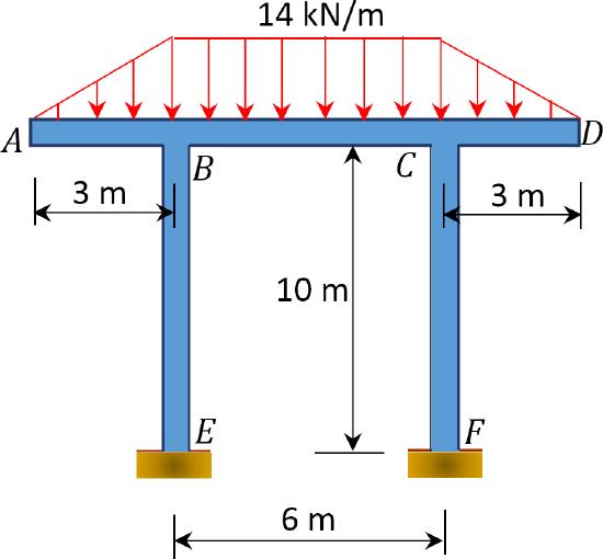
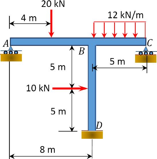
Example 12.5

Using the moment distribution method, determine the end moments at the supports of the frame shown in Figure 12.10. \(EI =\) constant.

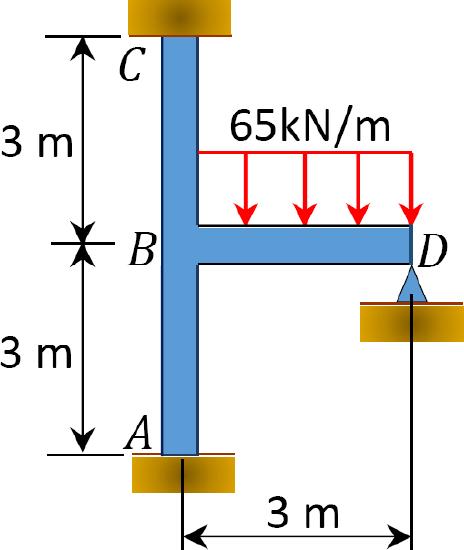
\(Fig. 12.10\). Frame.

Solution

Fixed end moment.

\(\begin{array}{l}
(F E M)_{A B}=(F E M)_{B A}=(F E M)_{B C}=(F E M)_{C B}=0 \\
(F E M)_{B D}=-\frac{w L^{2}}{12}=-\frac{65 \times 3^{2}}{12}=-48.75 \mathrm{kN} . \mathrm{m} \\
(F E M)_{D B}=\frac{w L^{2}}{12}=+48.75 \mathrm{kN} . \mathrm{m}
\end{array}\)

Stiffness factor.

\(\begin{array}{l}
K_{A B}=K_{B A}=\frac{I_{A B}}{L_{A B}}=\frac{I}{3}=0.333 \mathrm{I} \\
K_{B C}=K_{C B}=\frac{I_{B C}}{L_{B C}}=\frac{1}{3}=0.333 \mathrm{I} \\
K_{B D}=K_{D B}=\frac{3}{4} \times \frac{I_{B D}}{L_{B D}}=\frac{3}{4} \times \frac{\mathrm{I}}{3}=0.25 \mathrm{I}
\end{array}\)

Distribution factor.

\(\begin{array}{l}
(D F)_{A B}=0 \\
(D F)_{B A}=\frac{K_{B A}}{\sum K}=\frac{K_{B A}}{K_{B A}+K_{B C}+K_{B D}}=\frac{0.333 \mathrm{I}}{0.3331+0.3331+0.251}=0.36 \\
(D F)_{B C}=\frac{K_{B C}}{\sum K}=\frac{K_{B A}}{K_{B A}+K_{B C}+K_{B D}}=\frac{0.333 \mathrm{I}}{0.3331+0.3331+0.25 \mathrm{l}}=0.36 \\
(D F)_{C B}=0 \\
(D F)_{B D}=\frac{K_{B D}}{\sum K}=\frac{K_{B D}}{K_{B A}+K_{B C}+K_{B D}}=\frac{0.25 \mathrm{l}}{0.3331+0.333 \mathrm{I}+0.25 \mathrm{I}}=0.27 \\
(D F)_{D B}=\frac{K_{D B}}{\sum K}=\frac{K_{D B}}{K_{D B}+0}=\frac{0.25 \mathrm{l}}{0.251+0}=1
\end{array}\)

\(Table 12.5\). Distribution table.

Joint	A	B			C	D
Member	AB	BA	BC	BD	CB	DB
DF	0	0.36	0.36	0.27	0	1
FEM Dist. 1		-17.55	-17.55	+48.75 -13.16		-48.75 +48.75
CO Dist. 2	-8.78	-8.78	-8.78	+24.38 -6.58	-8.78
CO	-4.39				-4.39
Total	-13.17	-26.33	-26.33	+53.39	-13.17	0

Final member end moments.

\(\begin{array}{l}
M_{A B}=-13.17 \mathrm{k} . \mathrm{ft} \\
M_{B A}=-26.33 \mathrm{k} . \mathrm{ft} \\
M_{B C}=-26.33 \mathrm{k} . \mathrm{ft} \\
M_{B D}=+53.39 \mathrm{k} . \mathrm{ft} \\
M_{C B}=-13.17 \mathrm{k} . \mathrm{ft} \\
M_{D B}=0
\end{array}\)

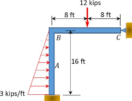
Example 12.6

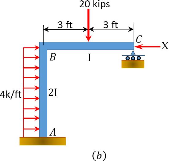
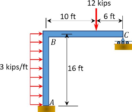
Using the moment distribution method, determine the member end-moments of the frame with side-sway shown in Figure 12.11a.

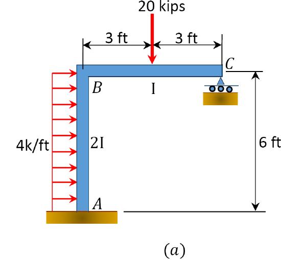
\(Fig. 12.11\). Frame with side – sway.

Solution

Fixed end moment.

\(\begin{array}{l}
(F E M)_{A B}=-\frac{w L^{2}}{12}=-\frac{4 \times 6^{2}}{12}=-12 \mathrm{k} . \mathrm{ft} \\
(F E M)_{B A}=\frac{w L^{2}}{12}=+12 \mathrm{k} . \mathrm{ft} \\
(F E M)_{B C}=-\frac{P L}{8}=-\frac{20 \times 6}{8}=-15 \mathrm{k.ft} \\
(F E M)_{C B}=+15 \mathrm{k} . \mathrm{ft}
\end{array}\)

Stiffness factor.

\(\begin{array}{l}
K_{A B}=K_{B A}=\frac{I_{A B}}{L_{A B}}=\frac{2 \mathrm{I}}{6}=0.333 \mathrm{I} \\
K_{B C}=K_{C B}=\frac{I_{B C}}{L_{B C}}=\frac{3}{4} \times \frac{1}{6}=0.125 \mathrm{I}
\end{array}\)

Distribution factor.

\(\begin{array}{l}
(D F)_{A B}=\frac{K_{A B}}{\sum K}=\frac{K_{A B}}{K_{A B}+\infty}=\frac{0.333 \mathrm{I}}{0.333 \mathrm{I}+\infty}=0 \\
(D F)_{B A}=\frac{K_{B A}}{\sum K}=\frac{K_{B A}}{K_{B A}+K_{B C}}=\frac{0.333 \mathrm{I}}{0.333 \mathrm{I}+0.125 \mathrm{I}}=0.73 \\
(D F)_{B C}=\frac{K_{B C}}{\sum K}=\frac{K_{B C}}{K_{B A}+K_{B C}}=\frac{0.125 \mathrm{I}}{0.333 \mathrm{I}+0.125 \mathrm{I}}=0.27 \\
(D F)_{C B}=\frac{K_{C B}}{\sum K}=\frac{K_{C B}}{K_{C B}+0}=\frac{0.125 \mathrm{I}}{0.125 \mathrm{I}+0}=1
\end{array}\)

Analysis of frame without side-sway.

\(Table 12.6\). Distribution table (no sway frame).

Joint	A	B		C
Member	AB	BA	BC	CB
DF	0	0.73	0.27	1
FEM Bal. 1	-12	+12 +2.19	-15 +0.81	+15 -15
CO Bal. 2	+1.095	+5.475	-7.5 +2.025
CO	+2.738
Total	-8.17	+19.67	-19.67	0

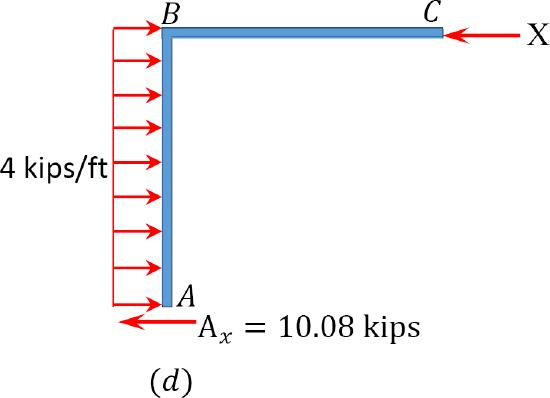
\(\begin{array}{l}
\sum M_{B}=0 \\
8.17+(4)(6)(3)-19.67-6 A_{x}=0 \\
A_{x}=\frac{[8.17+(4)(6)(3)-19.67]}{6}=10.08 \mathrm{kips} \\
\sum F_{x}=0 \\
(4)(6)-10.08-X=0 \\
X=13.92 \mathrm{kips}
\end{array}\)

Analysis of frame with side-sway.

Assume that \(M_{A B}=+20 \mathrm{k} . \mathrm{ft}\)

\(Table 12.7\). Distribution table (sway frame).

Joint	A	B		C
Member	AB	BA	BC	CB
DF	0	0.73	0.27	1
FEM Bal. 1	+20	+20 -14.6	-5.4
CO	-7.3
Total	+12.7	+5.4	-5.4	0

\(\begin{array}{l}
\qquad M_{B}=0 \\
-12.7-5.4+6 A_{x}=0 \\
A_{x}=\frac{(12.7+5.4)}{6}=3.02 \mathrm{kips}
\end{array}\)

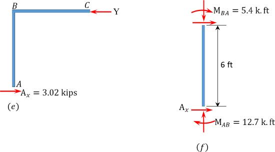
\(\begin{array}{l}
\sum F_{x}=0 \\
3.02-Y=0 \\
Y=3.02 \mathrm{kips} \\
\text { Corrective factor } \eta=\frac{x}{\mathrm{Y}}=\frac{13.92}{3.02}=4.61
\end{array}\)

Final end moments.

\(\begin{array}{l}
M_{A B}=-8.17+(12.7)(4.61)=50.38 \mathrm{k} . \mathrm{ft} \\
M_{B A}=19.67+(5.4)(4.61)=44.56 \mathrm{k} . \mathrm{ft} \\
M_{B C}=-19.67+(-5.4)(4.61)=-44.56 \mathrm{k} . \mathrm{ft} \\
M_{C B}=0
\end{array}\)

Example 12.7

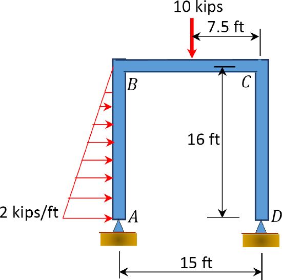
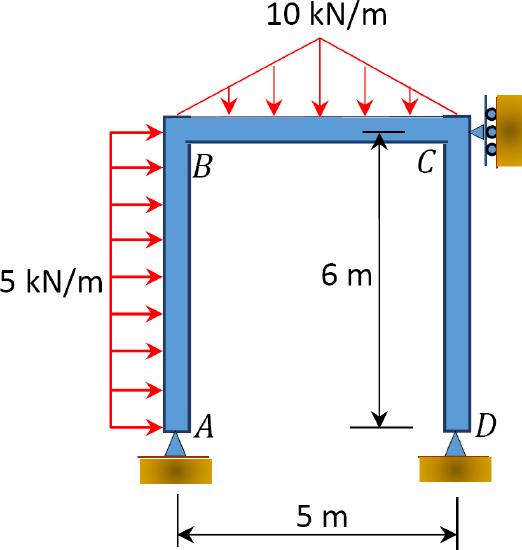
A sway frame is loaded as shown in Figure 12.12a. Using the moment distribution method, determine the end moments of the members of the frame.

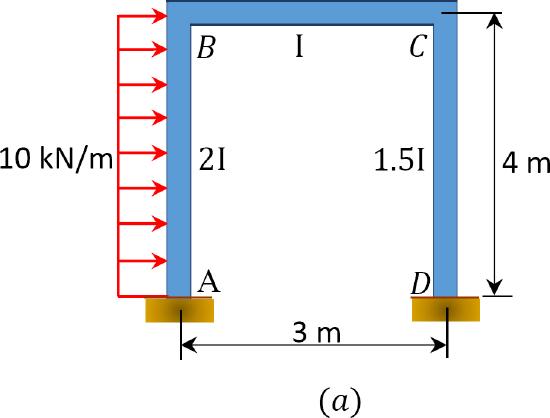
\(Fig. 12.12\). Loaded sway frame.

Solution

Fixed end moment.

\(\begin{array}{l}
(F E M)_{A B}=-\frac{w L^{2}}{12}=-\frac{10 \times 4^{2}}{12}=-13.33 \mathrm{kN} . \mathrm{m} \\
(F E M)_{B A}=\frac{w L^{2}}{12}=+13.33 \mathrm{kN} . \mathrm{m}
\end{array}\)

Stiffness factor.

\(\begin{array}{l}
K_{A B}=K_{B A}=\frac{I_{A B}}{L_{A B}}=\frac{2 \mathrm{I}}{4}=0.5 \mathrm{I} \\
K_{B C}=K_{C B}=\frac{I_{B C}}{L_{B C}}=\frac{I}{3}=0.333 \mathrm{I} \\
K_{C D}=K_{D C}=\frac{I_{B D}}{L_{B D}}=\frac{1.5 \mathrm{I}}{4}=0.375 \mathrm{I}
\end{array}\)

Distribution factor.

\(\begin{array}{l}
(D F)_{A B}=\frac{K_{A B}}{\sum K}=\frac{K_{A B}}{K_{A B}+0}=\frac{0.5 \mathrm{I}}{0.5 \mathrm{I}+\infty}=0 \\
(D F)_{B A}=\frac{K_{B A}}{\sum K}=\frac{K_{B A}}{K_{B A}+K_{B C}}=\frac{0.5 \mathrm{I}}{0.5 \mathrm{I}+0.333 \mathrm{I}}=0.60 \\
(D F)_{B C}=\frac{K_{B C}}{\sum K}=\frac{K_{B C}}{K_{B A}+K_{B C}}=\frac{0.333 \mathrm{I}}{0.333 \mathrm{I}+0.5}=0.40 \\
(D F)_{C B}=\frac{K_{C B}}{\sum K}=\frac{K_{C B}}{K_{C B}+K_{C D}}=\frac{0.333 \mathrm{I}}{0.333 \mathrm{I}+0.375 \mathrm{I}}=0.47 \\
(D F)_{C D}=\frac{K_{C D}}{\sum K}=\frac{K_{C D}}{K_{C B}+K_{C D}}=\frac{0.375 \mathrm{I}}{0.333 \mathrm{I}+0.375 \mathrm{I}}=0.53 \\
(D F)_{D C}=\frac{K_{D C}}{\sum K}=\frac{0.375 I}{0.375 I+\infty}=0
\end{array}\)

Analysis of frame without side-sway.

\(Table 12.8\). Distribution table (no sway frame).

Joint	A	B		C		D
Member	AB	BA	BC	CB	CD	DC
DF	0	0.60	0.4	0.47	0.53	0
FEM Dist. 1	-13.33	+13.33 -8.00	-5.33
CO Dist. 2	-4.00			-2.67 +1.25	+1.42
CO Dist. 3		-0.38	+0.63 -0.25			+0.71
CO Dist. 4	-0.19			-0.13 +0.06	+0.07
CO						+0.04
Total	-17.52	+4.95	-4.95	-1.49	+1.49	+0.75

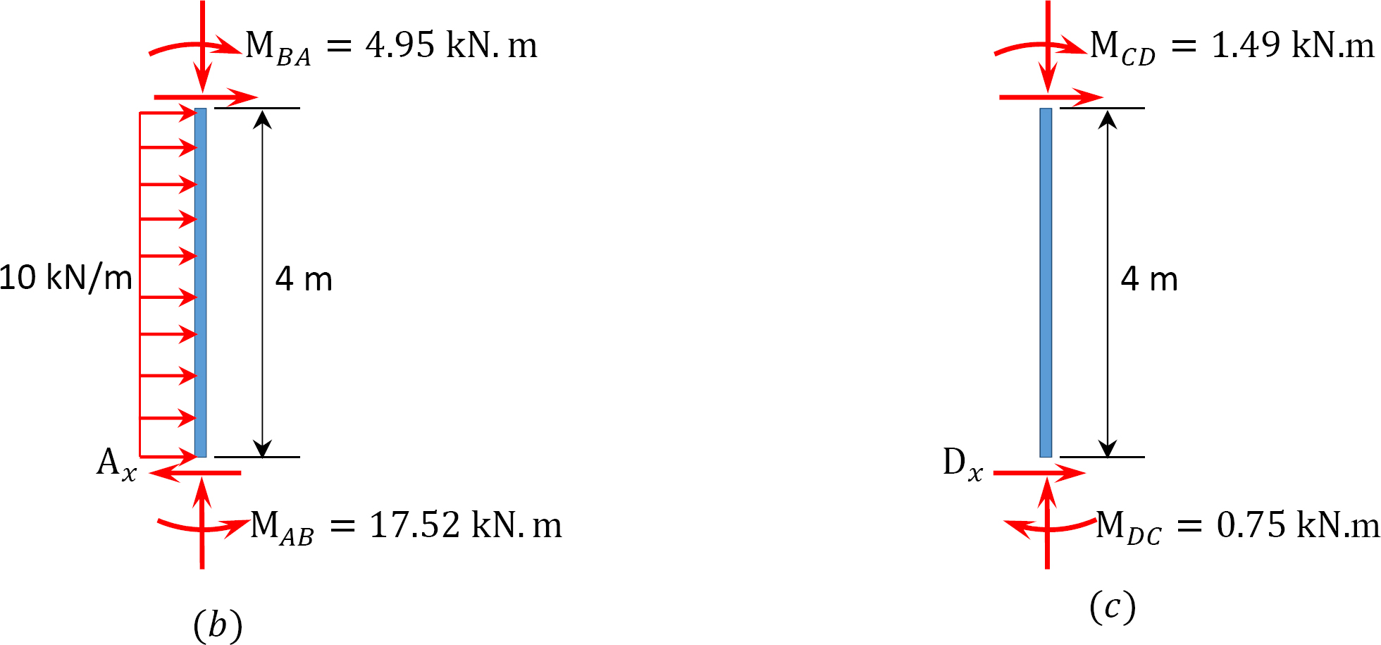
\(\begin{array}{l}
A_{x}=\frac{[17.52-4.95+(10)(4)(2)]}{4}=23.14 \mathrm{kN} \\
D_{x}=\frac{1.49+0.75}{4}=0.59 \mathrm{kN}
\end{array}\)

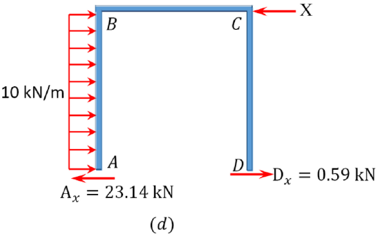
\(X=(10)(4)+0.59-23.14=17.45 \mathrm{kN}\)

\(Table 12.9\). Distribution table (sway frame).

Joint	A	B		C		D
Member	AB	BA	BC	CB	CD	DC
DF	0	0.6	0.40	0.47	0.53	0
FEM Dist. 1	+133	+133 -79.8	-53.2	-47.0	+100 -53.0	+100
CO Dist. 2	-39.9	+14.1	-23.5 +9.40	-26.6 +12.50	+14.10	-26.5
CO Dist. 3	+7.05	-3.75	+6.25 -2.50	+4.7 -2.21	-2.49	+7.05
CO Dist. 4	-1.88	+0.67	-1.11 0.44	-1.25 +0.59	+0.66	-1.25
CO Dist. 5	+0.34	-0.18	+0.30 -0.12	+0.22 -0.10	-0.12	+0.33
CO Dist. 6	-0.09	+0.03	-0.05 +0.02	-0.06 +0.03	+0.03	-0.06
Total	+98.52	+64.07	-64.07	-59.18	+59.18	+79.57

Analysis of frame with side-sway.

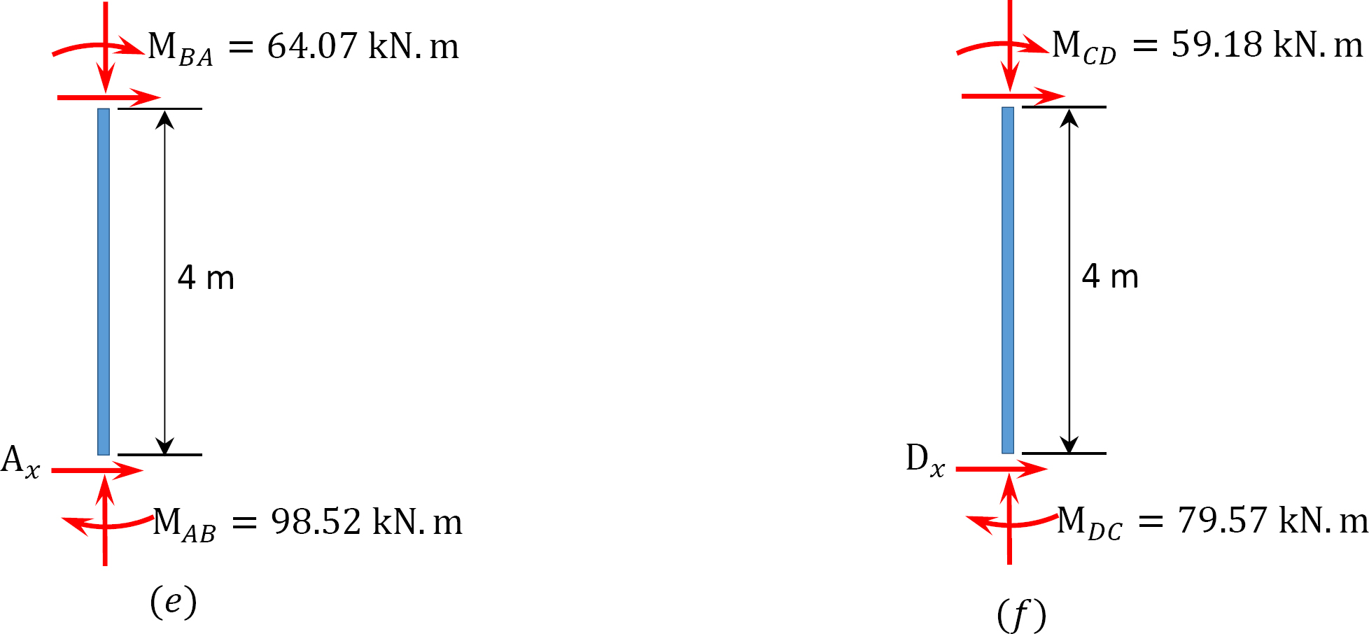
\(\begin{array}{l}
A_{x}=\frac{98.52+64.07}{4}=40.65 \mathrm{kN} \\
D_{x}=\frac{79.57+59.18}{4}=34.69 \mathrm{kN}
\end{array}\)

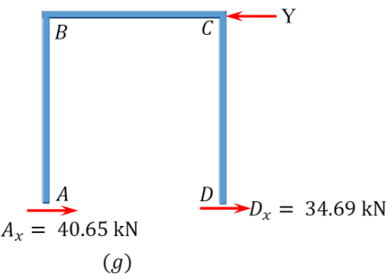
\(\begin{array}{l}
Y=40.65+34.69=75.34 \mathrm{kN} \\
\eta=\frac{X}{\mathrm{Y}}=\frac{17.45}{75.34}=0.23
\end{array}\)

Final end moment.

\(\begin{array}{l}
M_{A B}=-17.52+(98.52)(0.23)=5.14 \mathrm{kN} . \mathrm{m} \\
M_{B A}=4.95+(64.07)(0.23)=19.69 \mathrm{kN} . \mathrm{m} \\
M_{B C}=-4.95+(-64.07)(0.23)=-19.69 \mathrm{kN} . \mathrm{m} \\
M_{C B}=-1.49+(-59.18)(0.23)=-15.10 \mathrm{kN} . \mathrm{m} \\
M_{C D}=1.49+(59.18)(0.23)=15.10 \mathrm{kN} . \mathrm{m} \\
M_{D C}=0.75+(79.57)(0.23)=19.05 \mathrm{kN} . \mathrm{m}
\end{array}\)

Chapter Summary

Moment distribution method of analysis of indeterminate structures: The moment distribution method of analysis is an approximate method of analysis. Its degree of accuracy is dependent on the number of iterations. In this method, it is assumed that all joints in a structure are temporarily locked or clamped and, thus, are prevented from possible rotation. Loads are applied to the members, and the moments developed at the member ends due to fixity are determined. Joints in the structure are then unlocked successively, and the unbalanced moment at each joint is distributed to members meeting at that joint. Carry over moments at members’ far ends are determined, and the process of balancing is continued until the desired level of accuracy. Members’ end moments are determined by adding up the fixed-end moment, the distributed moment, and the carry over moment. Once members’ end moments are determined, the structure becomes determinate.

Practice Problems

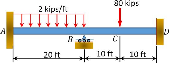
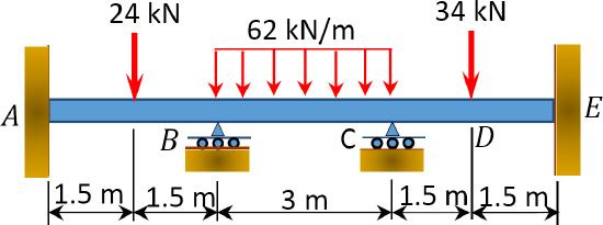
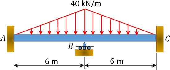
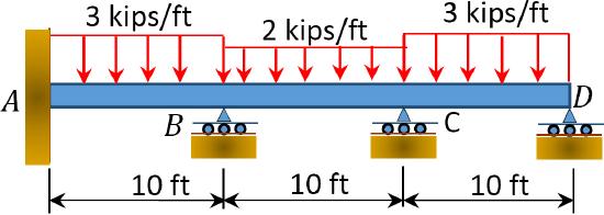
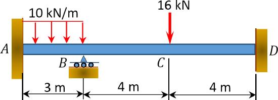
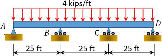
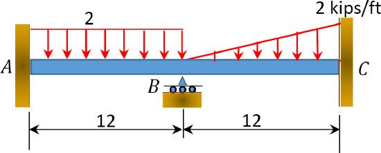
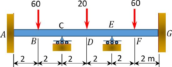
12.1 Use the moment distribution method to compute the end moment of members of the beams shown in Figure P12.1 through Figure P12.12 and draw the bending moment and shear force diagrams. \(EI = \)constant.

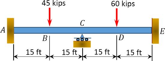
\(Fig. P12.1\). Beam.

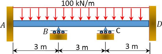
\(Fig. P12.2\). Beam.

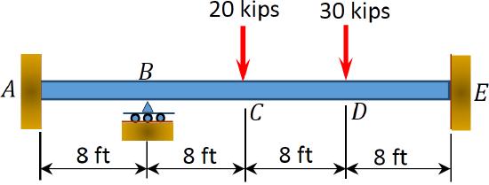
\(Fig. P12.3\). Beam.

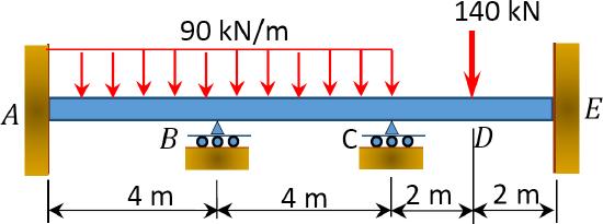
\(Fig. P12.4\). Beam.

\(Fig. P12.5\). Beam.

\(Fig. P12.6\). Beam.

\(Fig. P12.7\). Beam.

\(Fig. P12.8\). Beam.

\(Fig. P12.9\). Beam.

\(Fig. P12.10\). Beam.

\(Fig. P12.11\). Beam.

\(Fig. P12.12\). Beam.

12.2 Use the moment distribution method to compute the end moment of the members of the frames shown in Figure P12.13 through Figure 12.20 and draw the bending moment and shear force diagrams. \(EI = \)constant.

\(Fig. P12.13\). Frame.

\(Fig. P12.14\). Frame.

\(Fig. P12.15\). Frame.

\(Fig. P12.16\). Frame.

\(Fig. P12.17\). Frame.

\(Fig. P12.18\). Frame.

\(Fig. P12.19\). Frame.

\(Fig. P12.20\). Frame.