13.2: Static Equilibrium Method

Last updated
Save as PDF

Page ID: 43006

\( \newcommand{\vecs}[1]{\overset { \scriptstyle \rightharpoonup} {\mathbf{#1}} } \) \( \newcommand{\vecd}[1]{\overset{-\!-\!\rightharpoonup}{\vphantom{a}\smash {#1}}} \)\(\newcommand{\id}{\mathrm{id}}\) \( \newcommand{\Span}{\mathrm{span}}\) \( \newcommand{\kernel}{\mathrm{null}\,}\) \( \newcommand{\range}{\mathrm{range}\,}\) \( \newcommand{\RealPart}{\mathrm{Re}}\) \( \newcommand{\ImaginaryPart}{\mathrm{Im}}\) \( \newcommand{\Argument}{\mathrm{Arg}}\) \( \newcommand{\norm}[1]{\| #1 \|}\) \( \newcommand{\inner}[2]{\langle #1, #2 \rangle}\) \( \newcommand{\Span}{\mathrm{span}}\) \(\newcommand{\id}{\mathrm{id}}\) \( \newcommand{\Span}{\mathrm{span}}\) \( \newcommand{\kernel}{\mathrm{null}\,}\) \( \newcommand{\range}{\mathrm{range}\,}\) \( \newcommand{\RealPart}{\mathrm{Re}}\) \( \newcommand{\ImaginaryPart}{\mathrm{Im}}\) \( \newcommand{\Argument}{\mathrm{Arg}}\) \( \newcommand{\norm}[1]{\| #1 \|}\) \( \newcommand{\inner}[2]{\langle #1, #2 \rangle}\) \( \newcommand{\Span}{\mathrm{span}}\)\(\newcommand{\AA}{\unicode[.8,0]{x212B}}\)

To construct the influence line for the reaction at the prop of the cantilever beam shown in Figure 13.1, first determine the degree of indeterminacy of the structure. For the propped cantilever, the degree of indeterminacy is one, as the beam has four reactions (three at the fixed end and one at the prop). Thus, the propped cantilever has one reaction more than the three equations of equilibrium. Considering the reaction at the prop as the redundant and removing it from the system provides the primary structure. The next step is to apply a unit load at various distances \(x\) from the fixed support and at the position where the redundant was removed. Then, compute the deflections at these points on the beam using any method. The redundant \(B_{y}\) at the prop can be determined using the following compatibility equation:

\[\delta_{B X}+\delta_{B B} B_{Y}=0\]

From which

\[B_{y}=-\frac{\delta_{B X}}{\delta_{B B}}\]

where

\(\delta_{B X}\) = deflection at \(B\) due to the unit load at any arbitrary point on the primary structure at a distance \(x\) from the fixed support.
\(\delta_{B B}\) = deflection at \(B\) due to the unit value of the redundant (i.e., \(B_{y} = 1\)).

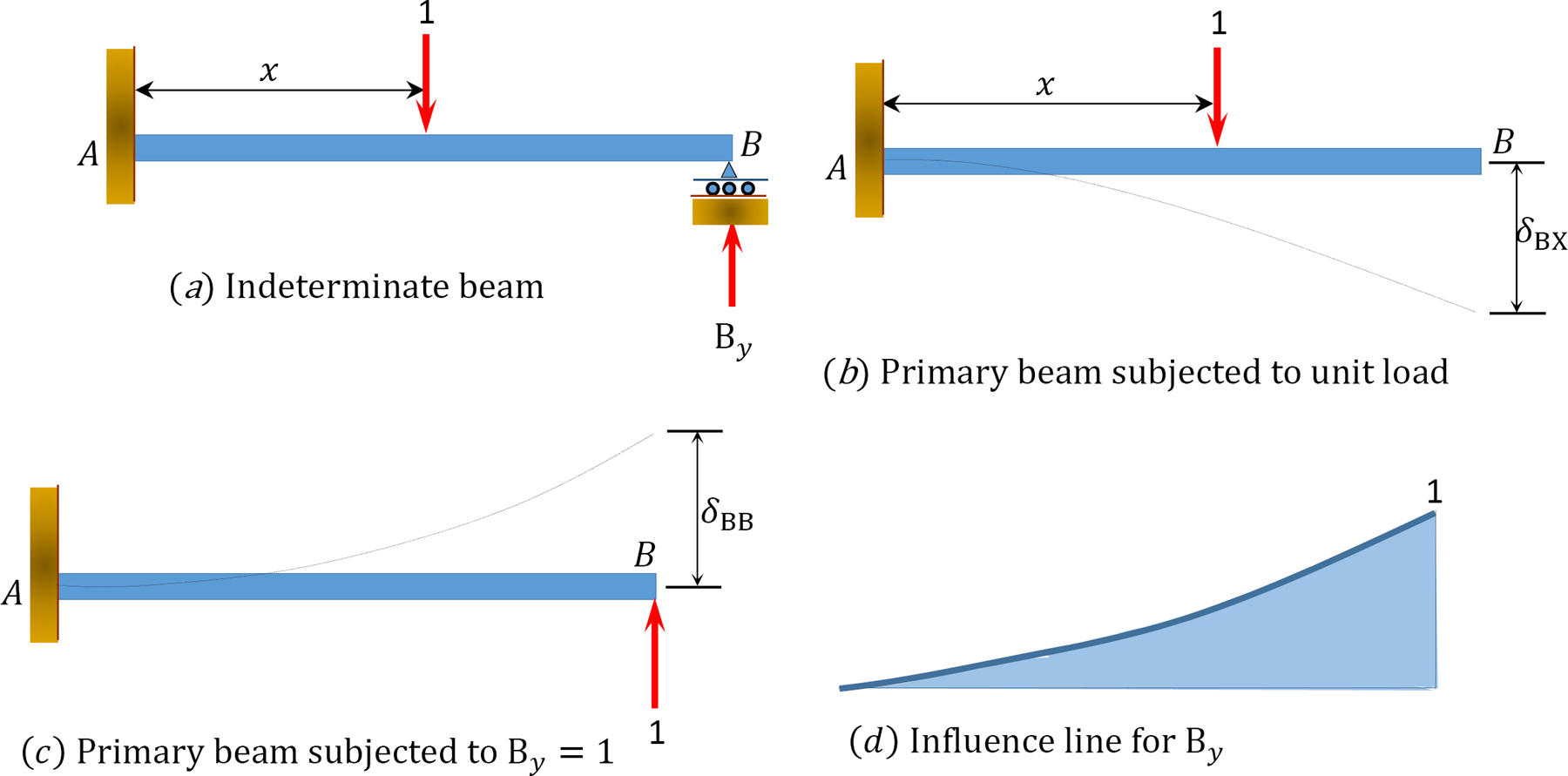
\(Fig. 13.1\). Cantilever beam.

Example \(\PageIndex{1}\)

Draw the influence lines for the reactions at supports \(A\) and \(B\) and the moment and shear force at point \(C\) of the propped cantilever beam shown in Figure 13.2a.

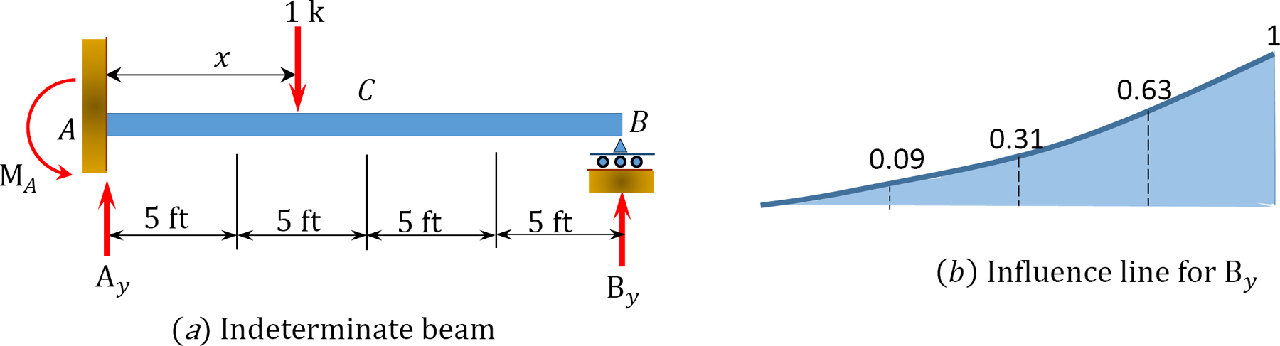
\(Fig. 13.2\). Propped cantilever beam.

Solution

The degree of indeterminacy of the beam is one. By selecting the reaction at the prop as the redundant, the value of this redundant can be determined by solving the following compatibility equation when the unit load is located at any point \(x\) along the beam:

\[\delta_{B X}+\delta_{B B} B_{Y}=0 \nonumber\]

Therefore,

\[B_{y}=-\frac{\delta_{B X}}{\delta_{B B}} \nonumber\]

Using the deflection formulas provided in appendix \(A\) of this book, the deflections at the prop due to a unit load acting at a quarter span interval along the beam can be determined as follows:

\(\begin{array}{l}
\delta_{B X}=\frac{P}{6 E I}\left(x^{3}-60 x^{2}\right) \\
\delta_{B 1}=\delta_{\mathrm{BA}}=0 \\
\delta_{B 2}=-229.17 \\
\delta_{B 3}=-833.33
\delta_{B 4}=-1687.5 \\
\delta_{B 5}=-2666.67 \\
\delta_{B B}=-\delta_{B 5}=2666.67
\end{array}\)

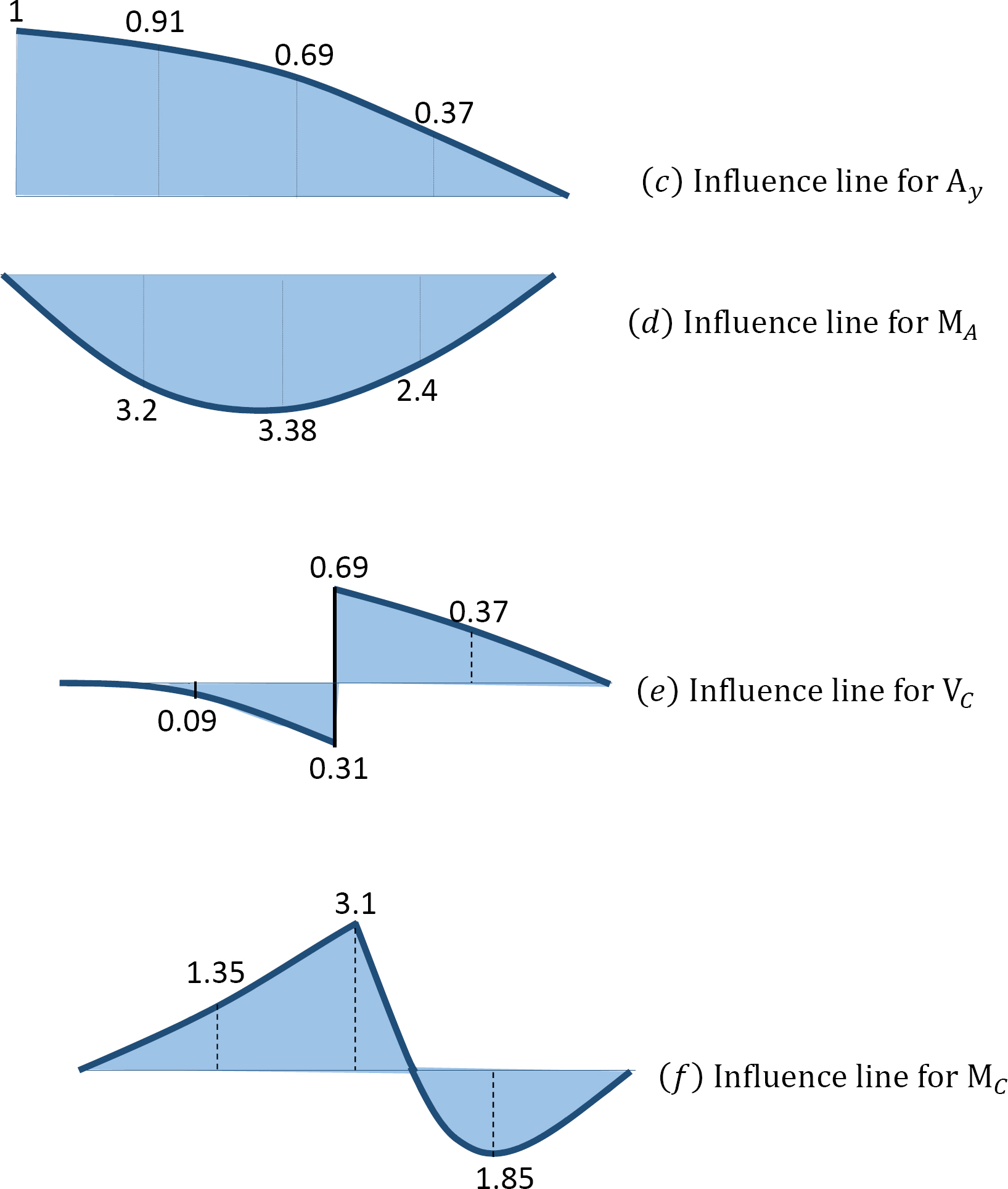
The ordinates of the influence lines for the desired functions are tabulated in Table 13.1

Table 13.1
x(ft)	(EI)\(\delta_B\)	B_y	A_y	M_A	V_C	M_C
0	0	0	1	0	0	0
5	-229.17	0.09	0.91	-3.2	-0.09	1.35
10	-833.33	0.31	0.69	-3.8	-0.31(L) 0.69 (R)	3.1
15	-1687.5	0.63	0.37	-2.4	0.37	-1.85
20	-2666.67	1	0	0	0	0

Example 13.2

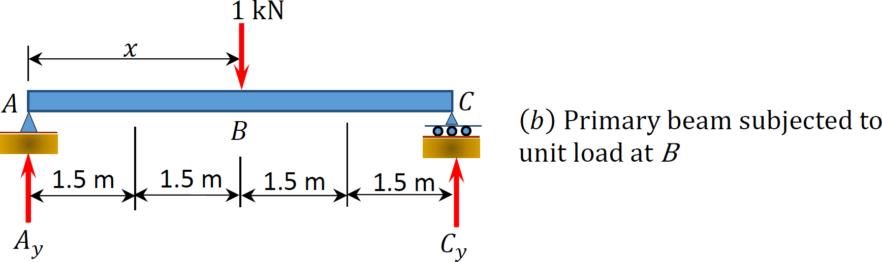
Draw the influence lines for the reactions at the supports \(A\), \(B\), and \(C\) of the indeterminate beam shown in Figure 13.3.

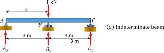
\(Fig. 13.3\). Indeterminate beam.

Solution

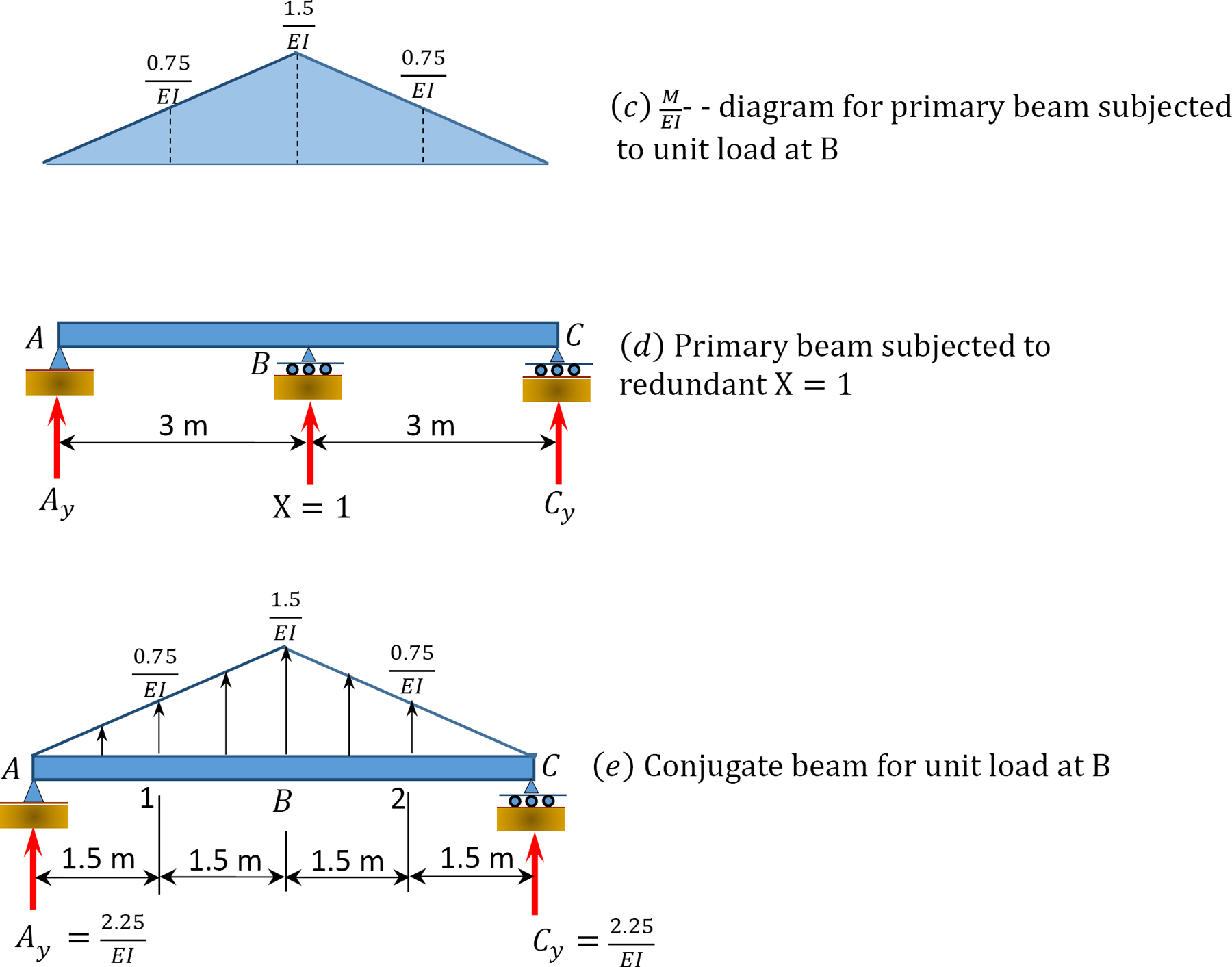
\(\begin{array}{c}
\delta_{\mathrm{BA}}=\delta_{\mathrm{BC}}=0 \\
\delta_{\mathrm{B} 1}=\delta_{\mathrm{B} 2}=\left(\frac{2.25}{E I}\right)(1.5)-\left(\frac{1}{2}\right)(1.5)\left(\frac{0.75}{E I}\right)\left(\frac{1.5}{3}\right)=3.09 \\
\delta_{\mathrm{BB}}=\left(\begin{array}{c}
2.25 \\
\overline{E I}
\end{array}\right)(3)-\left(\frac{1}{2}\right)(3)\left(\frac{1.5}{E 1}\right)\left(\frac{3}{3}\right)=4.50 \\
\delta_{\mathrm{BX}}=-\delta_{\mathrm{BB}}=-4.5
\end{array}\)

When the unit load is at different points along the beam, the ordinate of the influence line for the redundant at \(B_{y}\) can be computed using the compatibility equation:

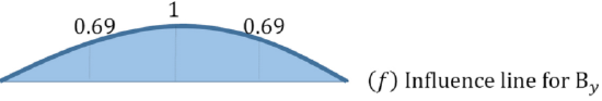
\(\begin{aligned}
&B_{y}=-\frac{\delta_{B X}}{\delta_{B B}} \\
&\text { At point } A \text { and } C, B_{y}=0 \\
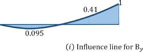
&\text { At point } 1 \text { and } 2, B_{y}=\frac{3.09}{45}=0.69 \\
&\text { At point } B, B_{y}=\frac{4.5}{4.5}=1.0
\end{aligned}\)

Now that \(B_{y}\) is known, the values of the ordinate of the influence lines for other reactions can be obtained using statics. For instance, to determine the ordinate of the influence line at point 1, place the unit load at point 1 and the value of the redundant when the unit load is at point 1 and solve as follows:

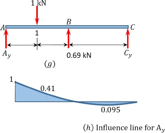
Ordinates of influence line for \(A_{y}\).

\(+ \curvearrowleft \sum M_{C}=0\)

When the unit load is at point 1,

\(\begin{aligned}
-A_{y}(6)+1(4.5)-0.69(3)=0 \\
A_{y}=\frac{2.43}{6}=0.41 \\
\end{aligned}\)

When the unit load is at point 2,

\(\begin{array}{l}
-A_{y}(6)+1(1.5)-0.69(3)=0 \\
A_{y}=\frac{2.43}{6}=-\frac{0.57}{6}=-0.095
\end{array}\)

When the unit load is at point \(A\), \(A_{y} = 1\)

When the unit load is at point \(B\) and \(C\), \(A_{y} = 0\)

Ordinates of Influence line for \(C_{y}\).

\(+ \curvearrowleft \sum M_{A}=0\)

When the unit load is at point 1,

\(\begin{aligned}
C_{y}(6)-1(1.5)+0.69(3)=0 \\
C_{y}=-\frac{0.57}{6}=-0.095 \\
\end{aligned}\)

When the unit load is at point 2,

\(\begin{array}{l}
C_{y}(6)-1(4.5)+0.69(3)=0 \\
A_{y}=\frac{2.43}{6}=0.41
\end{array}\)

When the unit load is at point \(C\), \(C_{y} = 1\)

When the unit load is at point \(A\) and \(B\), \(C_{y} = 0\)