3.1: Coordinate Systems and Frames of Reference

Every robot assumes a position in the real world that can be described by its position (x, y and z) and orientation (pitch, yaw and roll) along the three major axes of a Cartesian Coordinate system (See also Section 2.3, “Degrees of freedom”).

Figure \(\PageIndex{1}\): A coordinate system indicating the direction of the coordinate axes and rotation around them. These directions have been derived using the right-hand rules.

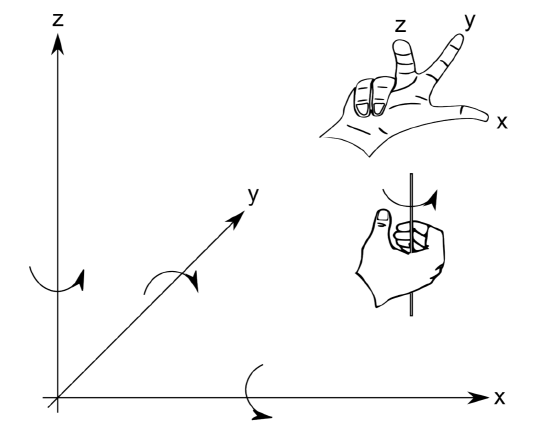
Such a coordinate system is shown in Figure 3.1.1. Note that the directions and orientations of the coordinate axes are arbitrary. This book uses the “right hand rules”, which are illustrated in Figure 3.1.1 to determine axes labels and directions throughout. Pitch, yaw, and roll, are also known as bank, attitude, and heading in other communities. This makes sense, considering the colloquial use of the word “heading”, which corresponds to a rotation around the z-axis of a vehicle driving on the x-y plane.

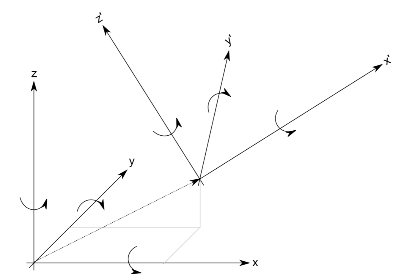
Defining all three position axes and orientations might be cumbersome. What level of detail we care about, where the origin of this coordinate system is, and even what kind of coordinate system we choose, depends on the specific application. For example, a simple mobile robot would typically require a representation with respect to a room, a building, or the earth’s coordinate system (given by the longitude and latitude of each point on the earth), whereas a static manipulator usually has the origin of its coordinate system at its base. More complicated systems, such as mobile manipulators or multi-legged robots, make life much easier by defining multiple coordinate systems, e.g. one for each leg and one that describes the position of the robot in the world frame. These local coordinate systems are known as Frames of Reference. An example of two nested coordinate systems is shown in Figure 3.1.2. In this example, a robot located at the origin of x^' , y^' and z^' might plan its motions in its own reference frame, which can then be expressed in the coordinate system x, y and z by performing a translation and a rotation as we will later see.

Figure \(\PageIndex{2}\): Two nested coordinate systems (frames of reference).

Depending on its degrees-of-freedom, that is the number of independent translations and rotations a robot can achieve in Cartesian space, it is also customary to ignore components of position and orientation that remain constant. For example a simple floor-cleaning robot’s pose might be completely defined by its x and y coordinates in a room as well as its orientation, i.e. its rotation around the z-axis.

3.1.1. Matrix notation

Given some kind of fixed coordinate system, we can describe the position of a robot’s end-effector by a 3x1 position vector. As there can be many coordinate systems defined on a robot and the environment, we identify the coordinate system a point relates to by a preceeding super-script, e.g., ^AP to indicate that point P is in coordinate system {A}. Each point consists of three elements ^AP = [p_xp_yp_z]^T .

More formally, ^AP is a linear combination of the three basis vectors that span A:

\[_{}^{A}\textrm{P}=p_{x}\begin{pmatrix}
1\\
0\\
0
\end{pmatrix}+p_{y}\begin{pmatrix}
0\\
1\\
0
\end{pmatrix}+p_{z}\begin{pmatrix}
0\\
0\\
1
\end{pmatrix}\]

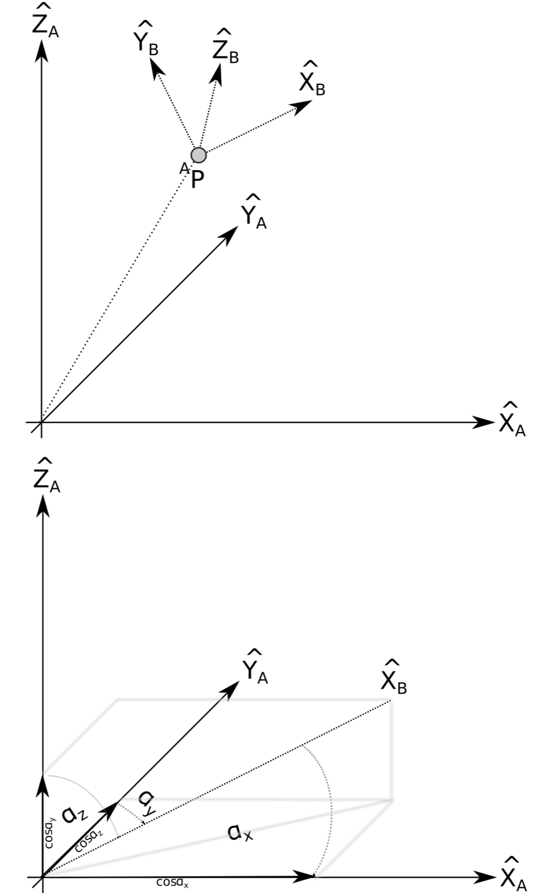
As we know, not only the position of the robot is important, but also its orientation. In order to describe the orientation of a point, we will attach a coordinate system to it. Let X̂_B , Ŷ_B and Ẑ_B be unit vectors that correspond to the principal axes of a coordinate system {B}. When expressed in coordinate system {A}, they are denoted ^AX̂_B, ^AŶ_B and ^AẐ_B. In order to express a vector that is given in one coordinate system in another, we need to project each of its components to the unit vectors that span the target coordinate system. For example considering only the axis ^AX̂_B

\[_{}^{A}\textrm{}X̂{_{B}}^{}=\left ( X̂{_{B}}^{}.X̂{_{A}}^{}, X̂{_{B}}^{}. Ŷ{_{A}}^{}, X̂{_{B}}^{}.Ẑ{_{A}}^{} \right )^{T}\]

consists of the projections of X̂_B onto X̂_A, Ŷ_A and Ẑ_A. Here, | · | denotes the scalar product (also known as dot or inner product). Note that all vectors in (3.1.2) are unit vectors, i.e. their length is one. By definition of the scalar product, A · B = ||A|| ||B|| cos α = cos α, indeed reduces the projection of X̂_B onto the unit vectors of {A}. This projection is illustrated in Figure 3.1.3.

Figure \(\PageIndex{3}\): Top: A coordinate system {B} with position given by ^AP and orientation given by X̂_B, Ŷ_B, and Ẑ_B. Bottom: The projection of the unit vector X̂_B onto the unit vectors that span coordinate system {A} after moving {B} into the origin of {A}. As all vectors are unit vectors, A · B = ||A|| ||B|| cos α = cos α.

We can now do this for all three vectors that span coordinate system {B} and stack these three vectors together into a 3x3 matrix to obtain the rotation matrix

\[_{B}^{A}\textrm{R}=\begin{bmatrix}
_{}^{A}X̂{_{B}}^{} & _{}^{A}Ŷ{_{B}}^{} & _{}^{A}Ẑ{_{B}}^{}
\end{bmatrix}\]

which describes {B} relative to {A}. It is important to note that all columns in _B^AR are unit vectors, so that the rotation matrix is orthonormal. This is important as this allows us to easily obtain the inverse of _B^AR as _B^AR^T or _A^BR =_B^AR^T .

Why the unit vectors of a coordinate system {B} expressed in coordinate system {A} actually make up a rotation matrix, can be easily seen when re-arranging Equation 3.1.1 in matrix form

\[_{}^{A}\textrm{P}=\begin{pmatrix}
1 & 0 & 0\\
0 & 1 & 0\\
0 & 0 & 1
\end{pmatrix} \begin{pmatrix}
p_{x}\\
p_{y}\\
p_{z}
\end{pmatrix}\]

where the rotation matrix is nothing but the identity as both points already are in the same coordinate system.

We have now established how to express the orientation of a coordinate system using a rotation matrix. Usually, coordinate systems don’t lie on top of each other, but are also displaced from each other. Together, position and orientation is known as a frame, which is a set of four vectors, one for the position and three for the orientation, and we can write

\[\left \{ B \right \}=\left \{ _{B}^{A}\textrm{R}, _{}^{A}\textrm{P}\right \}\]

to describe the coordinate frame {B} with respect to {A} using a vector ^AP and a rotation matrix _B^AR. Robots usually have many such frames defined along their bodies.

3.1.2. Mapping from one frame to another

Having introduced the concept of frames, we need the ability to map coordinates in one frame to coordinates in another frame. For example, let’s consider frame {B} having the same orientation as frame {A} and sitting at location ^AP in space. As the orientation of both frames is the same, we can express a point ^BQ in frame {A} as

\[_{}^{A}\textrm{Q}=_{}^{B}\textrm{Q}+_{}^{A}\textrm{P}\]

Actually, adding two vectors that are in different reference frames, i.e., ^BQ +^AP, is only possible if both of them have the same orientation. We can, however, convert from one reference frame to the other using the rotation matrix:

\[_{}^{A}\textrm{P}=_{B}^{A} \textrm{R}^{B}P\]

and therefore solve the mapping problem regardless of the orientation of {A} to {B}:

\[_{}^{A}\textrm{Q}=_{B}^{A} \textrm{R}^{B}Q+_{}^{A}\textrm{P}\]

Using this notation, we can see that leading subscripts cancel the leading superscripts of the following vector/rotation matrix. Whereas we have now a solution to transfer a point from one frame of reference to another by combining a rotation and a translation, it would be more appealing to write something like that:

_{}^{A}\textrm{Q}=_{B}^{A} \textrm{T}^{B}Q

In order to do this, we need to introduce a 4x1 position vector such that

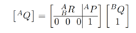
and _B^AT is a 4x4 matrix. Note that the added ‘1‘s and [0001] do not affect the other entries in the matrix during matrix multiplication. A 4x4 matrix of this form is called a homogenous transform.

The inverse of an homogeneous transform can be constructed by inverting rotation and translation part independently, leading to

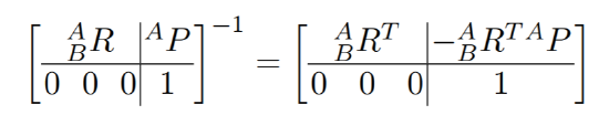
We have now established a convenient notation to convert points from one coordinate system to another. There are many possible ways this can be done, in particular how rotation can be represented (see below), but all can be converted from one into the other.

3.1.3. Transformation arithmetic

Transformations can be combined: consider for example an arm with two links, reference frame {A} at the base, {B} at its first joint, and {C} at its end-effector. Given the transforms _C^BT and _B^AT, we can write

\[_{}^{A}\textrm{P}=_{B}^{A}\textrm{T}_{C}^{B}\textrm{T}_{}^{C}\textrm{P}=_{C}^{A}\textrm{T}_{}^{C}\textrm{P}\]

to convert a point in the reference frame of the end-effector to that of its base. As this works for rotation and translation operators independently, we can construct _C^AT as

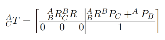
where ^AP_B and ^BP_C are the translations from {A} to {B} and from {B} to {C}, respectively.

3.1.4. Other representations for orientation

So far, we have represented orientation by a 3x3 matrix whose column vectors are orthogononal unit vectors describing the orientation of a coordinate system. Orientation is therefore represented with nine different values. We chose this representation mainly because it is the most intuitive to explain and is derived from simple geometry.

In fact, three values are sufficient to describe orientation. This becomes clear when considering that orthogonality (dot product of all columns is zero) and vector length (each vector must have length 1) impose six constraints on the nine values in the rotation matrix. Indeed, an orientation can be represented about a rotation by certain angles around the x, the y, and the z-axis of the reference coordinate system. This is known as the X − Y − Z fixed angle notation. Mathematically, this can be represented by a rotation matrix of the form

\[_{B}^{A}\textrm{R}_{XYZ(\gamma ,\beta ,\alpha )}=\begin{bmatrix}
\cos\alpha & -\sin\alpha & 0\\
\sin\alpha & \cos\alpha & 0\\
0 & 0 & 1
\end{bmatrix}\begin{bmatrix}
\cos\beta & 0 & \sin\beta \\
0 & 1 & 0\\
-\sin\beta & 0 & \cos\beta
\end{bmatrix}\begin{bmatrix}
1 & 0 & 0\\
0 & \cos\gamma & -\sin\gamma \\
0 & \sin\gamma & \cos\gamma
\end{bmatrix}\]

While the X −Y −Z fixed angles approach expresses a coordinate frame using rotations with respect to the original coordinate frame, say {A}, another possible description is to start with a coordinate frame {B} that is coincident with frame {A}, then rotate around the Z-axis with angle α, then the Y-axis with angle β and finally around the X-axis with angle γ. This representation is called Z-Y-X Euler angles. As the coordinate axis do not necessarily need to be different, there are twelve possible valid combinations of sub-sequent rotations:

XYX, XZX, YXY, YZY, ZXZ, ZYZ, XYZ, XZY, YZX, YXZ, ZXY and ZYX

There are only twelve, as sub-sequent rotations around the same axis are not valid. Such rotations would not add any information, but are equivalent to a rotation by the sum of both angles.

It is important to know about the subtle differences between the different available transformations as there is no “right” or “wrong”, but different manufacturers and fields use different conventions. There is only one caveat: each of the rotation matrices can look like subsequent rotations around the same axis for certain values of angles. For example, this happens for the XYZ rotation matrix if the angle of rotation around the Y-axis is 90° . These cases are known as a singularity.

Among these, the preferred representation for computational and stability reasons are Quaternions. A quaternion is a 4-tuple that extends the complex numbers with very general applications in mathematics and representing orientation and rotation in particular. The basic idea is that each rotation can be represented as a rotation around a single axis (a vector in space) by a specific angle. Given such an axis K = [k_xk_yk_z] T and an angle θ, one can calculate the so-called Euler parameters or unit quaternion:

\[\epsilon _{1}=k_{x}sin\frac{\theta }{2}\]

\[\epsilon _{2}=k_{y}sin\frac{\theta }{2}\]

\[\epsilon _{3}=k_{z}sin\frac{\theta }{2}\]

\[\epsilon _{4}=coz\frac{\theta }{2}\]

These four quantities are constrained by the relationship

\[\epsilon _{1}^{2}+\epsilon _{2}^{2}+\epsilon _{3}^{2}+\epsilon _{4}^{2}=1\]

which might be visualized by a point on a unit hyper-sphere. Analogous to rotation matrices, two quaternions ϵ_i and ϵ'_i can be multiplied using the following equation

\[\begin{pmatrix}
\epsilon _{4} & \epsilon _{1} & \epsilon _{2} & \epsilon _{3}\\
-\epsilon _{1}& \epsilon _{4} & -\epsilon _{3} &\epsilon _{2} \\
-\epsilon _{2} & \epsilon _{3} & \epsilon _{4} & -\epsilon _{1}^{c}\\
-\epsilon _{3}& -\epsilon _{2} & \epsilon _{1} & \epsilon _{4}
\end{pmatrix}\begin{pmatrix}
\epsilon _{4}^{'}\\
\epsilon _{1}^{'}\\
\epsilon _{2}^{'}\\
\epsilon _{3}^{'}
\end{pmatrix}\]

Unlike multiplying two rotation matrices, which requires 27 multiplications and 18 additions, multiplying two quaternions only requires 16 multiplications and 12 additions, making the operation computationally more efficient. In addition, the quaternion representation does not suffer from singularities for specific joint angles, making the approach computationally more robust.

Why any rotation can be expressed by a single vector can be seen when considering the properties of orthonomal rotation matrices. They have three Eigenvalues λ = 1 and a complex pair λ1,2 = cosθ ± i sinθ. Eigenvalues and Eigenvectors are defined as Rv = λv. For the case of λ = 1, the corresponding Eigenvector v is unchanged by rotation. This is only possible if v is the actual axis of rotation. The angle of rotation is now given by θ, which can be inferred from the complex pair.