3.2: Forward kinematics of selected Mechanisms

Now that we have introduced the notion of local coordinate frames, we are interested in how to calculate the pose and speed of these coordinate frames as a function of the robot’s actuators. We will first consider simple mechanisms where we can determine the relationship between actuators and the pose of various frames on the robot both in the position and speed domain. We will then consider the special class of non-holonomous mechanisms using a series of wheeled robots, for which the forward kinematics can only be calculated in the speed domain.

3.2.1. Forward kinematics of a simple arm

Figure \(\PageIndex{1}\): A simple 2-DOF arm.

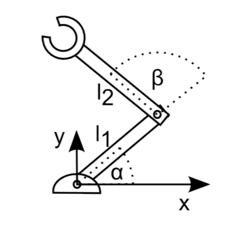
Consider a robot arm made out of two links and two joints that is mounted to a table. Let the length of the first link be l₁ and the length of the second link be l₂. You could specify the position of the link closer to the table by the angle α and the angle of the second link relative to the first link using the angle β. Suitable conventions and coordinate systems are shown in Figure 3.2.1.

We can now calculate the position of the joint between the first and the second link using simple trigonometry:

\[x_{1}=\cos\alpha l_{1}\]

\[y_{1}=\sin\alpha l_{1}\]

Similarly, the position of the end-effector is given by

\[x_{2}=\cos(\alpha +\beta )l_{2}+x_{1}\]

\[y_{2}=\sin(\alpha +\beta )l_{2}+y_{1}\]

or together, the position of the end-effector (x, y) is given by

\[x=\cos(\alpha +\beta)l_{2}+\cos\alpha l_{1}\]

\[y=\sin(\alpha +\beta)l_{2}+\sin\alpha l_{1}\]

The above equations are the kinematic equations of this robot as they relate its control parameters α and β to the position of its end-effector given in the local coordinate system spanned by x and y with the origin at the robot’s base. Note that both α and β shown in the figure are positive: Both links rotate around the z-axis. Using the right-hand rule, the direction of positive angles is defined to be counter-clockwise.

The configuration space,i.e., the set of angles each actuator can be set to, of this robot is given by −π/2 < α < π/2 as it is not supposed to run into the table, and −π < β < π. The configuration space is given with respect to the robot’s joints and allows us to calculate the workspace of the robot, i.e., the physical space it can move to, using the forward kinematic equations. This terminology will be identical for mobile robots. An example of configuration and work-space for both a manipulator and a mobile robot is shown in Figure 3.2.2.

The orientation of the arm’s end-effector is given by α+β. We can now write down a transformation that includes a rotation around the z-axis

\[\begin{pmatrix}
cos_{\alpha \beta } &-sin_{\alpha \beta } & 0 &\cos_{\alpha \beta }l_{2}+\cos\alpha l_{1} \\
sin_{\alpha \beta }& cos_{\alpha \beta } & 0 & \sin_{\alpha \beta }l_{2}+\sin\alpha l_{1}\\
0 & 0 & 1 & 0\\
0& 0 & 0 & 1
\end{pmatrix}\]

The notation sinαβ and cosαβ are short-hand for sin(α + β) and cos(α + β), respectively.

This transformation now allows us to translate from the robot’s base to the robot’s end-effector as a function of the actuator positions α and β. This transformation will be helpful if we want to calculate suitable joint angles in order to reach a certain pose or if we want to convert measurements taken relative to the end-effector back into the base’s coordinate system.

3.2.2. Forward Kinematics of a Differential Wheels Robot

Whereas the pose of a robotic manipulator is uniquely defined by its joint angles—which can be made available using encoders in almost real-time—this is not the case for a mobile robot. Here, the encoder values simply refer to wheel orientation and need to be integrated over time, which will be a huge source of uncertainty as we will later see. What complicates matters is that for so-called non-holonomic systems, it is not sufficient to simply measure the distance that each wheel traveled, but also when each movement was executed.

Figure \(\PageIndex{2}\): Configuration space (left) and workspace (right) for a non-holonomic mobile robot (top) and a holonomic manipulator (bottom). Closed trajectories in configuration space result in closed trajectories in the workspace if the robot’s kinematics is holonomic.

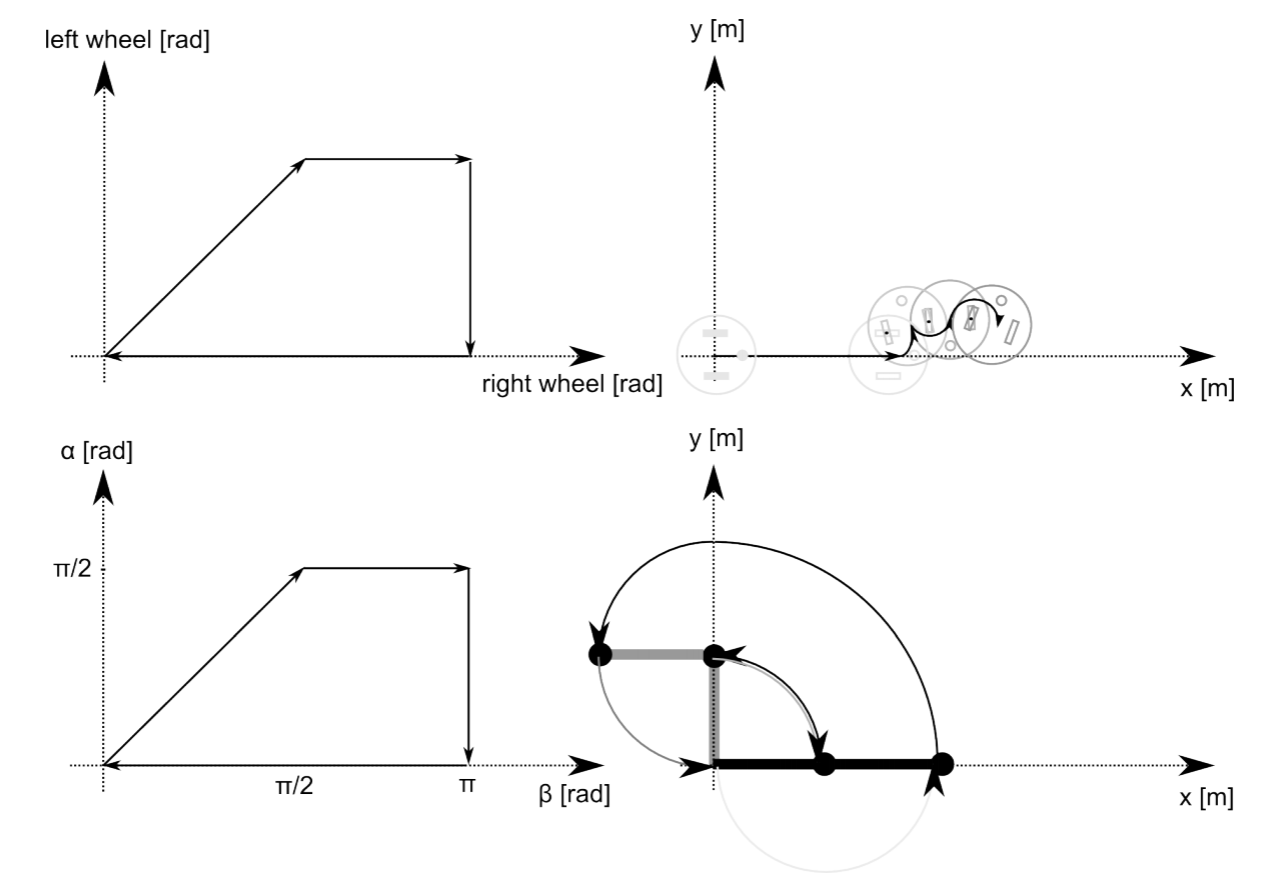
A system is non-holonomic when closed trajectories in its configuration space (reminder: the configuration space of a two-link robotic arm is spanned by the possible values of each angle) may not have it return to its original state. A simple arm is holonomic, as each joint position corresponds to a unique position in space. Going through whatever trajectory that comes back to the starting point in configuration space, will put the robot at the exact same position. A train on a track is holonomic: moving its wheels backwards by the same amount they have been moving forward brings the train to the exact same position in space. A car and a differential-wheel robot are non-holonomic vehicles: performing a straight line and then a right-turn leads to the same amount of wheel rotation than doing a right turn first and then going in a straight line; getting the robot to its initial position requires not only to rewind both wheels by the same amount, but also getting their relative speeds right. The configuration and corresponding workspace trajectories for a non-holonomic and a holonomic robot are shown in Figure 3.2.2. Here, a robot first moves on a straight line (both wheels turn an equal amount). Then the left wheel remains fixed and only the right wheel turns forward. Then the right wheel remain fixed and the left wheel turns backward. Finally, the right wheel turns backward, arriving at the initial encoder values (zero). Yet, the robot does not return to its origin. Performing a similar trajectory in the configuration space of a two-link manipulator instead, let the robot return to its initial position.

It should be clear by now that for a mobile robot, not only traveled distance per wheel matters, but also the speed of each wheel as a function of time. Instead, this information was not required to uniquely determine the pose of a manipulating arm. Let’s introduce the following conventions. We will establish a world coordinate system {I}, which is known as the inertial frame by convention (Figure 3.6). We establish a coordinate system {R} on the robot and express the robot’s speed ^Rξ as a vector

\[_{}^{R}\textrm{ξ} =\left [ _{}^{R}\textrm{x}, _{}^{R}\textrm{y},_{}^{R}\textrm{θ}\right ]^{T}\nonumber\]

Here R_x and R_y correspond to the speed along the x and y directions in {R}, whereas R_θ corresponds to the rotation around the imaginary z-axis, that you can imagine to be sticking out of the ground. We denote speeds with dots over the variable name, as speed is simply the derivative of distance. Think about the robot’s position in {R}. It is always zero, as the coordinate system is fixed on the robot. Therefore, velocities are the only interesting quantities in this coordinate system and we need to understand how velocities in {R} map to positions in {I}, which we denote by ^Iξ = [^Ix, ^Iy, ^Iθ]^T . These coordinate systems are shown in Figure 3.2.3.

Figure \(\PageIndex{3}\): Mobile robot with local coordinate system {R} and world frame {I}. The arrows indicate the positive direction of position and orientation vectors.

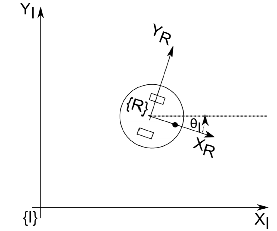
Notice that the positioning of the coordinate frames and their orientation are arbitrary. Here, we choose to place the coordinate system in the center of the robot’s axle and align ^Rx with its default driving direction.

In order to calculate the robot’s position in the inertial frame, we need to first find out, how speed in the robot coordinate frame maps to speed in the inertial frame. This can be done again by employing trigonometry. There is only one complication: a movement into the robot’s x-axis might lead to movement along both the x-axis and the y-axis of the world coordinate frame. By looking at the figure above, we can derive the following components to x_I . First,

\[x_{I,x}=cos(\theta)x_{R}\]

There is also a component of motion coming from ˙y_R (ignoring the kinematic constraints for now, see below). For negative θ, as in Figure 3.2.3, a move along y_R would let the robot move into positive X_I direction. The projection from ˙yR is therefore given by

\[x_{I,y}=-sin(\theta)y_{R}\]

We can now write

\[x_{I,y}=cos(\theta)x_{R}-sin(\theta)y_{R}\]

Similar reasoning leads to

\[y_{I}=sin(\theta)x_{R}+cos(\theta)y_{R}\]

and

\[\theta _{I}=\theta _{R}\]

which is the case because both robot’s and world coordinate system share the same z-axis in this example. We can now conveniently write

\[\xi _{I}=_{R}^{I}\textrm{T}(\theta )\xi _{R}\]

with

\[_{R}^{I}\textrm{T}(\theta )=\begin{pmatrix}
cos(\theta ) & -sin(\theta ) & 0\\
sin(\theta ) & cos(\theta ) & 0\\
0& 0 & 1
\end{pmatrix}\]

We are now left with the problem of how to calculate the speed ˙ ξ_R in robot coordinates. For this, we make use of the kinematic constraints of the robotic wheels. For a standard wheel, the kinematic constraints are that every rotation of the wheel leads to strictly forward or backward motion and does not allow side-way motion or sliding. We can therefore calculate the forward speed of a wheel x using its rotational speed φ (assuming the encoder value/angle is expressed as φ) and radius r by

\[x=\phi r\]

This becomes apparent when considering that the circumference of a wheel with radius r is 2πr. The distance a wheel rolls when turned by the angle φ (in radians) is therefore x = φr, see also Figure 3.2.4, right. Taking the derivative of this expression on both sides leads to the above expression.

Figure \(\PageIndex{4}\): Left: Differential wheel robot pivoting around its left wheel. Right: A wheel with radius r moves by φr when rotated by φ degrees.

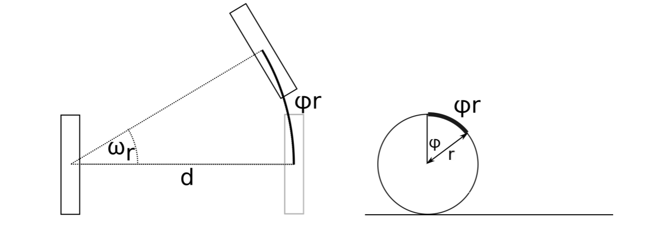
How each of the two wheels in our example contributes to the speed of the robot’s center—where its coordinate system is anchored—requires the following trick: we calculate the contribution of each individual wheel while assuming all other wheels remaining un-actuated. In this example, the distance traveled by the center point is exactly half of that traveled by each individual wheel, assuming the non-actuated wheel rotating around its ground contact point (Figure 3.2.4). We can therefore write

\[x_{R}=\frac{r\phi _{l}}{2}+\frac{r\phi _{r}}{2}\]

given the speeds φ_l and φ_r of the left and the right wheel, respectively.

Note

Think about how the robot’s speed along its y-axis is affected by the wheel-speed given the coordinate system in the drawing above. Think about the kinematic constraints that the standard wheels impose.

Hard to believe at first, but the speed of the robot along its y-axis is always zero. This is because the constraints of the standard wheel tell us that the robot can never slide. We are now left with calculating the rotation of the robot around its zaxis. That there is such a thing can be immediately seen when imaging the robot’s wheels spinning in opposite directions. We will again consider each wheel independently. Assuming the left wheel to be non-actuated, spinning the right wheel forwards will lead to counter-clockwise rotation. Given an axle diameter (distance between the robot’s wheels) d, we can now write

\[\omega_{r}d=\phi_{r}r\]

with ω_r the angle of rotation around the left wheel (Figure 3.2.4, right). Taking the derivative on both sides yields speeds and we can write

\[\omega_{r}=\frac{\phi_{r}r}{d} \]

Adding the rotation speeds up (with the one around the right wheel being negative based on the right-hand grip rule), leads to

\[\omega_{r}=\frac{\phi_{r}r}{d}-\frac{\phi_{l}r}{d} \]

Putting it all together, we can write

\[\begin{pmatrix}
x_{I}\\
y_{I}\\
\theta
\end{pmatrix}=\begin{pmatrix}
cos(\theta) & -sin(\theta) & 0\\
sin(\theta) & cos(\theta) & 0\\
0 &0 &1
\end{pmatrix}\begin{pmatrix}
\frac{r\phi _{l}}{2}+\frac{r\phi _{r}}{2}\\
0\\
\frac{\phi _{r}r}{d}-\frac{\phi _{l}r}{d}
\end{pmatrix}\]

From Forward Kinematics to Odometry

Equation 3.2.20 only provides us with the relationship between the robot’s wheel-speed and its speed in the inertial frame. Calculating its actual pose in the inertial frame is known as odometry. Technically, it requires integrating (3.2.20) from 0 to the current time T. As this is not possible, but for very special cases, one can approximate the robot’s pose by summing up speeds over discrete time intervals, or more precisely

\[\begin{pmatrix}
x_{I}(T)\\
y_{I}(T)\\
\theta (T)
\end{pmatrix}=\int_{0}^{T}\begin{pmatrix}
x_{I}(t)\\
y_{I}(t)\\
\theta (t)
\end{pmatrix}dt\approx \sum_{k=0}^{k=T}\begin{pmatrix}
\Delta x_{I}(k)\\
\Delta y_{I}(k)\\
\Delta \theta (k)
\end{pmatrix}\Delta t\]

which can be calculated incrementally as

\[x_{I}(k+1)=x_{I}(k)+\Delta x(k)\]

using ∆x(k) ≈ x_I(t) and similar expressions for y_I and θ. Note that (3.2.22) is just an approximation. The larger ∆t becomes, the more inaccurate this approximation becomes as the robot’s speed might change during the interval.

Note

Don’t let the notion of an integral worry you! As robots’ computers are fundamentally discrete, integrals usually turn into sums, which are nothing than for-loops.

3.2.3. Forward kinematics of Car-like steering

Differential wheel drives are very popular in mobile robotics as they are very easy to build, maintain, and control. Although not holonomic, a differential drive can approximate the function of a fully holonomic robot by first driving on the spot to achieve the desired heading and then driving straight. Drawbacks of the differential drive are its reliance on a caster wheel, which performs poorly at high speeds, and difficulties in driving straight lines as this requires both motors to drive at the exact same speed.

These drawbacks are mitigated by car-like mechanisms, which are driven by a single motor and can steer their front wheels. This mechanism is known as “Ackermann steering”. Ackermann steering should not be confused with “turntable” steering where the front wheels are fixed on an axis with central pivot point. Instead, each wheel has its own pivot point and the system is constrained in such a way that all wheels of the car drive on circles with a common center point, avoiding skid. As the Ackermann mechanism lets all wheels drive on circles with a common center point, its kinematics can be approximated by those of a tricycle with rear-wheel drive, or even simpler by a bicycle. This is shown in Figure 3.2.5.

Figure \(\PageIndex{5}\): Left: Kinematics of car-like steering and the equivalent bicycle model. Right: Mechanism of an Ackermann vehicle.

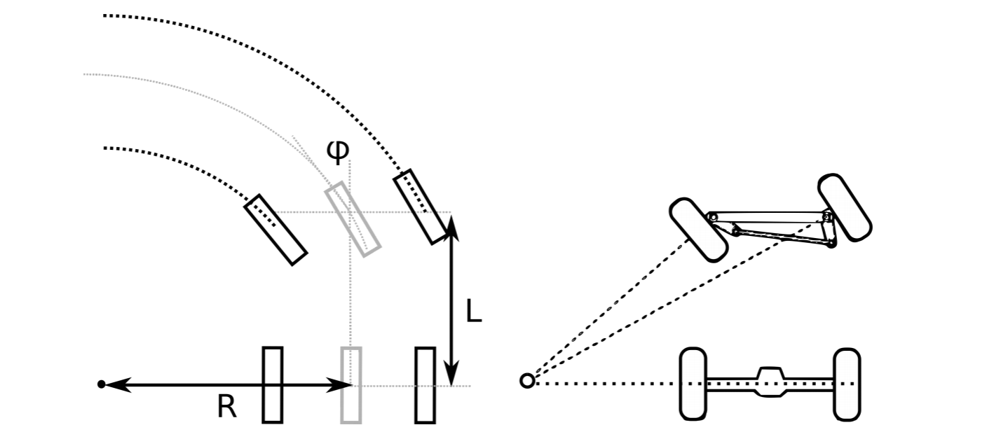
Let the car have the shape of a box with length L between rear and front axis. Let the center point of the common circle described by all wheels be distance R from the car’s longitudinal center line. Then, the steering angle φ is given by

\[\tan\phi =\frac{L}{R}\]

The angles of the left and the right wheel, φ_l and φ_r can be calculated using the fact that all wheels of the car rotate around circles with a common center point. With the distance between the two front wheels l, we can write

\[\frac{L}{R-l/2}=\tan(\pi /2-\phi _{r})\]

\[\frac{L}{R+l/2}=\tan(\pi /2-\phi _{l})\]

This is important, as it allows us to calculate the resulting wheel angles resulting from a specific angle φ and test whether they are within the constraints of the actual vehicle. Assuming the wheelspeed to be ω and the wheel radius r, we can calculate the speeds in the robot’s coordinate frame to

\[x_{r}=\omega _{r}\]

\[y_{r}=0\]

\[\theta _{r}=\frac{\omega r\tan\phi }{L}\]

using (3.2.23) to calculate the circle radius R.