3.5: Inverse Kinematics using Feedback-Control

Solving the inverse kinematic problem for non-holonomic mobile robots require us to find a sequence of actuation commands. One way of doing this is to employ feedback control. In a nutshell, feedback control uses the error between actual and desired position to calculate a trajectory piece that drives the robot a little closer to its desired pose. The process is then repeated until the error is marginally small. This approach can not only be used for mobile robots, but also for manipulator arms with kinematics that are too complicated to solve analytically.

3.5.1. Feedback control for mobile robots

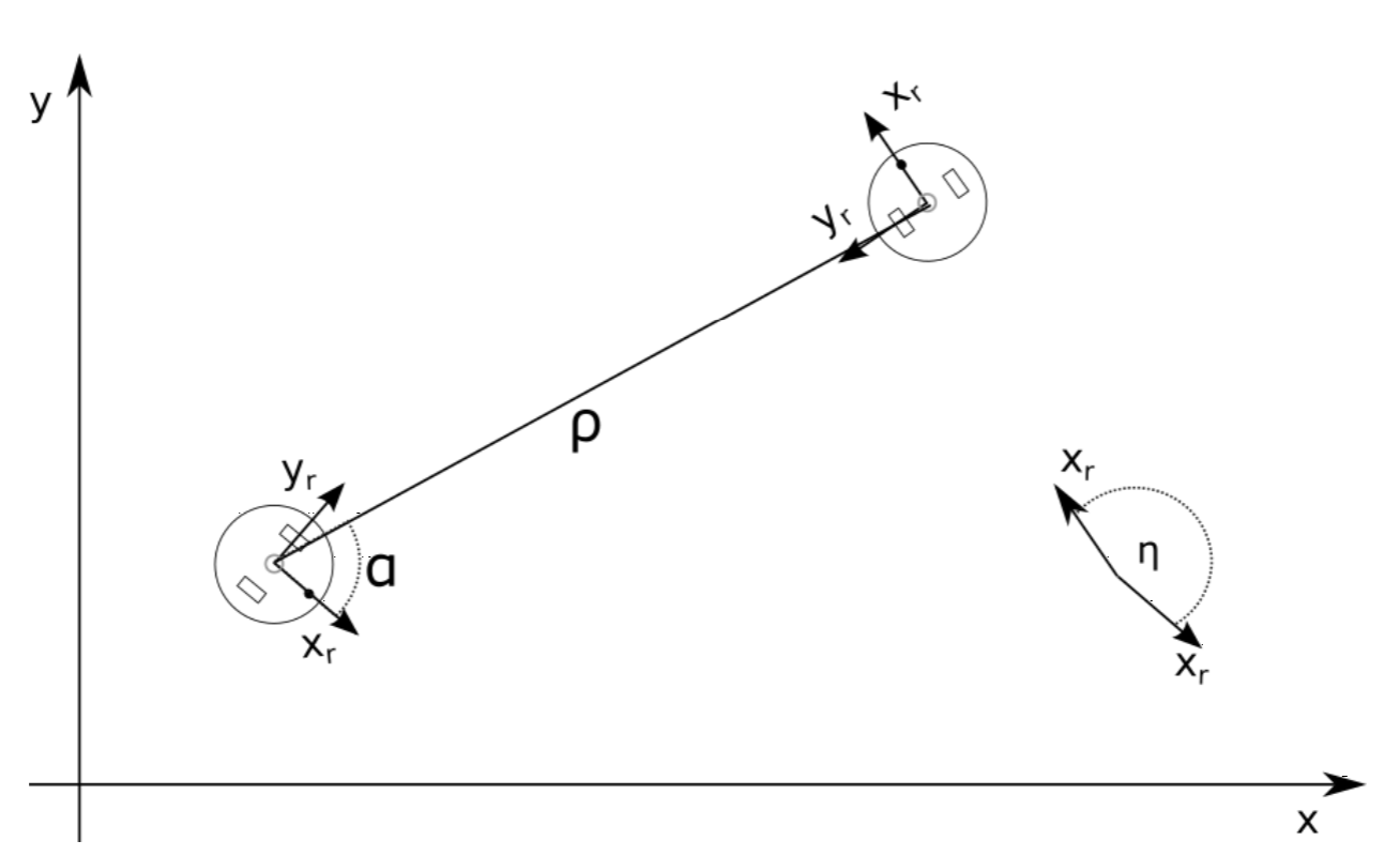
Assume the robot’s position given by x_r, y_r and θ_r and the desired pose as x_g, y_g and θ_g with the subscript g indicating “goal”. We can now calculate the error in the desired pose by

\[\rho =\sqrt{(x_{r}-x_{g})^{2}+(y_{r}-y_{g})^{2}}\]

\[\alpha =\tan^{-1}\frac{y_{g}-y_{r}}{x_{g}-x_{r}}-\theta _{r}\nonumber\]

\[\eta =\theta _{g}-\theta _{r}\nonumber\]

which is illustrated in Figure 3.5.1. These errors can be turned directly into robot’s speeds, for example using a simple proportional controller with gains p1, p2 and p3:

\[x=p_{1}\rho \]

\[\theta =p_{2}\alpha +p_{3}\eta\]

which will let the robot drive in a curve until it reaches the desired pose.

3.5.2. Inverse Jacobian Technique

Figure \(\PageIndex{1}\): Difference in desired and actual pose as a function of distance ρ, bearing α and heading η.

The two-link arm (Figure 3.2.1) involved only two free parameters, but was already pretty complex to solve analytically if the end-effector pose was not specified. One can imagine that things become very hard with more degrees of freedom or more complex geometries. (Mechanisms in which some axes intersect are simpler to solve than others, for example.) Fortunately, there are simple numerical techniques that work reasonably well. One of them known is as Inverse Jacobian technique:

As we can easily calculate the resulting pose for every possible joint angle combination using the forward kinematic equations, we can calculate the error between desired and actual pose. This error actually provides us with a direction that the end-effector needs to move. As we only need to move tiny bits at a time and can then re-calculate the error, this is an attractive method to generate a trajectory that moves the arm to where we want it go and thereby solving the inverse kinematics problem.

In order to do this, we need an expression that relates the desired speed of the robot’s end-effector, i.e., the direction in which we want to move, to the speed at which we need to change our joints. Let the translational speed of a robot be given by

\[\upsilon =\begin{pmatrix}
x\\
y\\
z
\end{pmatrix}\]

As the robot can potentially not only translate, but also rotate, we also need to specify its angular velocity. Let these velocities be given as a vector

\[\omega =\begin{pmatrix}
\omega _{x}\\
\omega _{y}\\
\omega _{z}
\end{pmatrix}\]

This notation is also called a velocity screw. We can now write translational and rotational velocities in a 6x1 vector as (v ω)^T. Let the joint angles/positions be j = (j₁, . . . , j_n).

Given a relationship between end-effector velocities j and joint velocities J, we can write

\[\begin{pmatrix}
\upsilon & \omega
\end{pmatrix}^{T}=J(j_{1},...,j_{n})^{T}\]

with n the number of joints. J is also known as the Jacobian matrix and contains all partial derivatives that relate every joint angles to every velocities. In practice, J looks like

\[\begin{pmatrix}
\upsilon \\
\omega
\end{pmatrix}=\begin{pmatrix}
\frac{∂x}{∂j_{1}} & \cdots & \frac{∂x}{∂j_{n}}\\
\vdots & &\vdots \\
\frac{∂\omega_{ z}}{∂j_{1}}& \cdots &\frac{∂\omega_{z}}{∂j_{n}}
\end{pmatrix}(j_{1},...,j_{n})^{T}\]

This notation is important as it tells us how small changes in the joint space will affect the end-effector’s position in cartesian space. Better yet, the forward kinematics of a mechanism can always be calculated, as well as their analytical derivatives, allowing us to calculate numerical values for the entries of matrix J for every possible joint angle/position.

It would now be desirable to just invert J in order to calculate the necessary joint speeds for every desired end-effector speeds. Unfortunately, J is only invertible if there are exactly 6 independent joints, so that J is quadratic and has full rank. If this is not the case, we can use the pseudo-inverse instead:

\[J^{+}=\frac{J^{T}}{JJ^{T}}=J^{T}(JJ^{T})^{-1}\]

As you can see, J^T cancels from the equation leaving 1/J, while being applicable to non-quadratic matrices.

This solution might or might not be numerically stable, depending on the current joint values. If the inverse of J is mathematically not feasible, we speak of a singularity of the mechanism. This happens for example when two joint axes line up, therefore effectively removing a degree of freedom from the mechanism, or at the boundary of the workspace. Mathematically speaking the rank of the Jacobian is smaller than six.

We can now write a simple feedback controller that drives our error e as the difference between desired and actual position to zero:

\[\Delta j=-J^{+}e\]

That is, we move each joint a tiny bit into the direction that minimizes e. It can be easily seen that the joint speeds are only zero if e has become zero. A problem arises, however, when the end-effector has to go through a singularity to get to its goal. Then, the solution to J⁺ “explodes” and joint speeds go to infinity. In order to work around this, we can introduce damping to the controller.

This can be achieved by not only minimizing the error, but also the joint velocities. Thus, the minimization problem becomes

\[\parallel J\Delta j-e\parallel +\lambda ^{2}\parallel \Delta j\parallel ^{2}\]

where λ is some constant. One can show that the resulting controller that achieves this has the form

\[\Delta j=(J^{T}J+\lambda ^{2}I)^{-1}J^{+}e\]

This is known as the Damped Least-Squares method. Problems with this approach are local minima and singularities of the mechanism, which might render this solution infeasible.