
3.4: Inverse Kinematics of Selected Mechanisms
- Page ID
- 14784

The forward kinematics of a system are given by a transformation matrix from the base of a manipulator (or a corner of the room) to the end-effector of a manipulator (or a mobile robot). As such, they are an exact description of the pose of the robot. In order to find the joint angles that lead to the desired pose, we will need to solve these equations for joint angles as a function of the desired pose. For a mobile robot, we can do this only for velocities in the local coordinate system, and need more sophisticated methods to calculate appropriate trajectories for the robot.
3.4.1. Solvability
As the resulting equations are heavily non-linear, it makes sense to briefly think about whether we can solve them at all for specific parameters before trying. Here, the workspace of a robot becomes important. The workspace is the sub-space that can be reached by the robot in any orientation. Clearly, there will be no solutions for the inverse kinematic problem outside of the workspace of the robot.
A second question to ask is how many solutions we actually expect and what it means to have multiple solutions geometrically. Multiple solutions to achieve a desired pose correspond to multiple ways in which a robot can reach a target. For example a three-link arm that wants to reach a point that can be reached without fully extending all links (leading to a single solution), can do this by folding its links in a concave and a convex fashion. How many solutions there are for a given mechanism and pose quickly becomes non-intuitive. For example a 6-DOF arm can reach certain points with up to 16 different conformations.
3.4.2. Inverse Kinematics of a Simple Manipulator Arm
We will now look at the kinematics of a 2-link arm that we introduced earlier. We need to solve the equations determining the robot’s forward kinematics by solving for α and β. This is tricky, however, as we have to deal with complicated trigonometric expressions.
To get an intuition, assume there to be only one link, l1. Solving (3.2.1) for α yields actually two solutions [cos−1 x1/l1 , − cos−1 x1/l1] , as cosine is symmetric for positive and negative values. Indeed, for any possible position on the x−axis ranging from −l1 to l1, there exist two solutions. One with the arm above the table, one with the arm within the table. (At the extremes of the workspace, both solutions are the same.)
Solving for both degrees of freedom actually yields eight solutions, of which only two are feasible:
\[\alpha \rightarrow \cos^{-1}\left ( \frac{x^{2}y+y^{3}-\sqrt{4x^{4}-x^{6}+4x^{2}y^{2}-2x^{4}y^{2}-x^{2}y^{4}}}{2(x^{2}+y^{2})} \right )\]
and
\[\beta \rightarrow -\cos^{-1}(1/2(-2)x^{2}+y^{2}))\]
What will drastically simplify this problem, is to not only specificy the desired position, but also the orientation of the end-effector. In this case, a desired pose can be specified by
\[\begin{pmatrix}
cos\phi & -sin\phi & 0 & x\\
sin\phi & cos\phi & 0 &y\\
0 & 0 & 1 & 0\\
0 & 0 & 0 & 1
\end{pmatrix}\]
A solution can now be found by simply equating the individual entries of the transformation (3.2.7) with those of the desired pose. Specifically, we can observe
\[cos\phi =cos(\alpha +\beta )\]
\[x=\cos_{\alpha \beta }l_{2}+\cos_{\alpha}l_{1}\nonumber\]
\[y=\sin_{\alpha \beta }l_{2}+\sin_{\alpha}l_{1}\nonumber\]
These can be reduced to
\phi =\alpha +\beta
\[\cos\alpha =\frac{\cos_{\alpha \beta }l_{2}-x}{l_{1}}=\frac{\cos_{\phi }l_{2}-x}{l_{1}}\nonumber\]
\[\sin\alpha =\frac{\sin{\alpha \beta }l_{2}-y}{l_{1}}=\frac{\sin_{\phi }l_{2}-y}{l_{1}}\nonumber\]
Providing the orientation of the robot in addition to the desired position therefore allows solving for α and β just as a function of x, y and φ.
As such solutions quickly become unhandy with more dimensions, however, you can calculate a numerical solution using an approach that we will later see is very similar to path planning in mobile robotics. One way to do this is to plot the distance of the end-effector from the desired solution in configuration space. To do this, you need to solve the forward kinematics for every point in configuration space and use the Euclidian distance to the desired target as height. In our example this would be
\[f_{x,y}(\alpha ,\beta )=\sqrt{(\sin(\alpha +\beta )+\sin(\alpha )-y)^{2}+(\cos(\alpha +\beta)+\cos(a)-x^{2})}\]
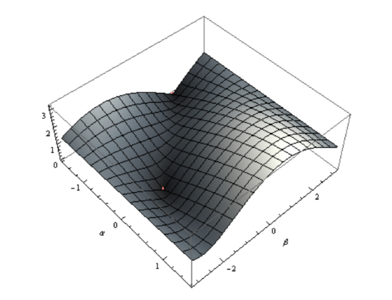
This is plotted for α = [−π/2, π/2] and β = [−π, π] and x = 1, y = 1 in Figure 3.4.1. This function has a minima, in this case zero, for values of α and β that bring the manipulator to (1, 1). These values are (α → 0, b → −π 2 ) and (α → −π 2 , b → π 2 ).
You can now think about inverse kinematics as a path finding problem from anywhere in the configuration space to the nearest minima. A formal approach to doing this will be discussed in Section 3.5. How to find shortest paths in space, that is finding the shortest route for a robot to get from A to B will be a subject of chapter 4.
3.4.3. Inverse Kinematics of Mobile Robots
As there is no unique relationship between the amount of rotation of a robot’s individual wheels and its position in space, but for simple holonomic platforms such as a robot on a track, we will treat the inverse kinematics problem at first only for the velocities of the local robot coordinate frame.
Let’s first establish how to calculate the necessary speed of the robot’s center given a desired speed ξI in world coordinates. We can transform the expression ξI = T(θ)ξR by multiplying both sides with the inverse of T(θ):
\[T^{-1}(\theta )\xi_{I}=T^{-1}(\theta)T(\theta)\xi _{R}\]
which leads to ξR = T−1 (θ)ξI. Here
\[T^{-1}=\begin{pmatrix}
cos\theta & sin\theta &0 \\
-sin\theta & cos\theta & 0\\
0 & 0 & 1
\end{pmatrix}\]
which can be determined by actually performing the matrix inversion or by deriving the trigonometric relationships from the drawing. Similarly, we can now solve
\[\begin{pmatrix}
x_{R}\\
y_{R}\\
\theta
\end{pmatrix}=\begin{pmatrix}
\frac{r\phi _{l}}{2}+\frac{r\phi _{r}}{2}\\
0\\
\frac{\phi _{r}r}{d}-\frac{\phi _{l}r}{d}
\end{pmatrix}\]
for φl , φr
\[\phi _{l}= (2x_{R}-\theta d)/2r\]
\[\phi _{r}= (2x_{R}+\theta d)/2r\]
allowing us to calculate the robot’s wheelspeed as a function of a desired xR and θ, which can be calculated using (3.4.6).
Note that this approach does not allow us to deal with yR ≠ 0, which might result from a desired speed in the inertial frame. Non-zero values for translation in y-direction are simply ignored by the inverse kinematic solution, and driving toward a specific point either requires feedback control (Section 3.5.2) or path planning (Chapter 4).